 WonksAnonymous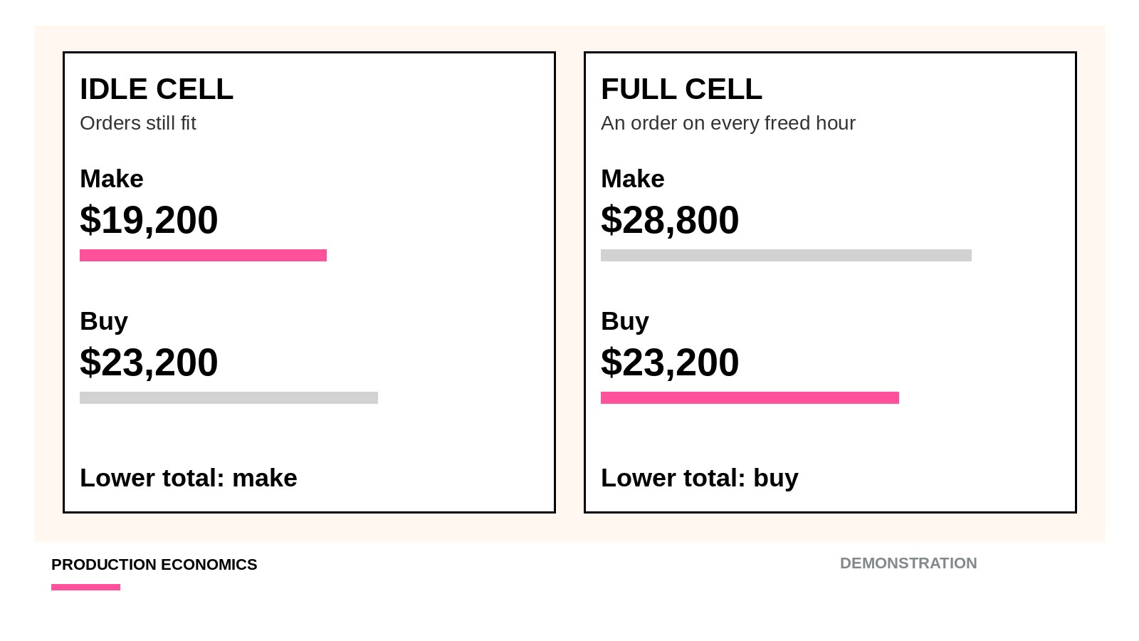
Make or Buy at a Bottleneck: Calculate the Opportunity Cost
Compare avoidable make cost with purchase-and-delivery cost, then add only the contribution of orders the same hours could ship.
An hour spent making a component can cost more than the routing shows. If that hour is how you would have shipped another order you already hold, add the contribution that order would earn, and add it only for units that order covers.
On spare hours, the make or buy relevant cost is the avoidable cost of making the component, set next to the cost to buy it and receive it. On a full cell, the make or buy opportunity cost is the contribution of the orders those hours could have shipped. Selling price stays out of that sum. A make or buy cost analysis here is those two totals, plus a stop at the last real order.
Scroll horizontally to see all columns.
| Idle cell | Full cell, with an order for every freed hour | |
|---|---|---|
| Relevant cost to make | Avoidable make cost | Avoidable make cost + contribution given up |
| Relevant cost to buy | Purchase price + freight and receiving | The same purchase-and-delivery cost |
| Opportunity cost | $0 | Contribution per constrained hour x hours that have orders |
| Unavoidable costs | Flag them. Leave them out of both columns | Flag them. Leave them out of both columns |
| Lower total | Make, when avoidable make cost is lower | Buy, when the freed contribution exceeds the extra purchase cost |
The lower relevant total is the cost answer for the hours you entered. Quality, delivery, and how long the quote lasts sit outside the table. The dollars further down are a demonstration you can recompute. They are teaching inputs, not a quote, a benchmark, or a named company’s costs.
Count only the costs that change
A cost is relevant when it differs between making the component and buying it. OpenStax, in section 10.1 of Principles of Managerial Accounting, calls a cost avoidable when choosing the other option removes it, and unavoidable when it remains for the short run either way. A sunk cost has already been spent, so it is the same under both choices.
Section 10.3 applies that split to a component. Materials, direct labor, and variable overhead of making the component exist only if you make it. Fixed cost that continues after you buy drops out. Fixed cost that ends when you buy, such as overtime supervision tied to that job, stays in the make column. The relevant costs for a make or buy decision are those lines, plus the purchase-and-delivery cost on the buy side.
Avoidable make cost = materials
                     + direct labor that stops if you buy
                     + variable overhead that stops if you buy
                     + fixed cost that stops if you buy

Purchase-and-delivery cost = supplier price
                            + inbound freight
                            + receiving and incoming inspection
Mark each line before you add it.
Scroll horizontally to see all columns.
| Line | Does it change if you buy? | Where it goes |
|---|---|---|
| Materials, job labor, variable overhead | Yes | Avoidable make cost |
| A fixed cost that ends with the job | Yes | Avoidable make cost |
| Rent, depreciation of machines you keep, allocated plant overhead | No | Unavoidable flag. Neither column |
| Tooling or a setup already paid | Already spent | Sunk. Neither column |
| Supplier price, freight, receiving | Yes, and only if you buy | Purchase-and-delivery cost |
Allocated overhead still appears on an absorption-cost report. It does not move with this choice. Folding it into the make column, or into the buy column, creates a gap the cash does not have. Fixed, variable, and total cost is the sort to do before you mark the lines.
Takeaway: Put a changing cost in one column. Flag an unavoidable cost and leave it out of both.
Spare hours add no opportunity cost
Opportunity cost is the benefit of the alternative you do not take. On an idle cell that benefit is zero when making the component still leaves enough hours for every order the cell could ship, or when the cell has no such order.
Idle relevant cost to make = avoidable make cost
Idle relevant cost to buy  = purchase-and-delivery cost
Opportunity cost            = 0
Choose the lower of those two. Section 10.3 states the idle-cell rule this way: when qualitative issues do not override the numbers, buy if the purchase price is below the avoidable cost of making. The calculation in that section does not add a second product. It does note that buying can free capacity, and section 10.6 prices that freed time at contribution per constrained hour.
Takeaway: Hours that no order is waiting on add $0 to the cost of making.
A full cell adds contribution per constrained hour, and then stops
Section 10.6 defines unit contribution margin as selling price minus variable cost per unit. Contribution per unit of the scarce resource is that margin divided by the amount of the constraint the unit uses. When one product still has demand you cannot fill, the value of another hour on the constraint is that contribution per hour. The chapter lists outsourcing at the bottleneck as one way to free the constraint.
Contribution per unit = selling price - variable cost per unit

Contribution per constrained hour = contribution per unit
                                   / constrained hours per unit

Opportunity cost = contribution per constrained hour
                   x hours that would ship an order you already have

Full-cell cost to make = avoidable make cost + opportunity cost
Full-cell cost to buy  = purchase-and-delivery cost
The demand ceiling is the quantity on those orders. Hours past the ceiling have no contribution to add. A forecast, a sales target, or empty time on the schedule does not raise it.
Contribution is the rate, because the units you skip also skip their variable cost. Measuring the Cost of Unplanned Production Downtime uses that same split when a sold-out line stops: lost contribution when the packs had a buyer, and selling price only as an upper bound. The constraint is the stage that limits what you can ship, as in Why Faster Machines Do Not Always Increase Line Output.
This page uses one other product. Ranking several products by contribution per constrained hour, each up to its own orders, is a separate product-mix decision. The tables below do not make that ranking.
Takeaway: Multiply contribution per constrained hour by the hours that have orders. Stop at the last order.
Demonstration: 800 components on one cell
Every dollar and hour in this section is a demonstration. The inputs are round so you can multiply them again. They are not a supplier quote, a market price, a benchmark, or a cost taken from a real company. Swap in your order book and your cost records before you treat a total as a decision.
Scroll horizontally to see all columns.
| Input | Demonstration | What you enter |
|---|---|---|
| Components required this period | 800 | Your requirement |
| Materials per component | $12 | Bill of material |
| Direct labor per component, paid only if you make it | $6 | Routing |
| Variable overhead per component | $4 | Costs that move with the component |
| Fixed cost per component that stops if you buy | $2 | The fixed line that actually ends |
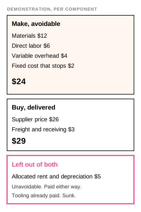
| Allocated rent and depreciation per component | $5 | Unavoidable flag. Leave it out |
| Tooling already paid | Sunk | Leave it out |
| Supplier price per component | $26 | The quote, and the period it covers |
| Freight and receiving per component | $3 | Inbound cost |
| Constrained hours per component | 0.25 | Hours on the constraint |
| Other product, selling price | $80 | Order price |
| Other product, variable cost | $32 | Cost avoided if you do not run it |
| Other product, constrained hours per unit | 1 | Hours on the same constraint |
| Hours available on the cell | 400 in the idle case, 200 in the full case | Your schedule |
| Orders in hand for the other product | Set in each case below | Confirmed orders only |
Avoidable make cost per component = 12 + 6 + 4 + 2 = $24.
Purchase-and-delivery = 26 + 3 = $29.
Contribution of the other product = 80 - 32 = $48 per unit.
Contribution per constrained hour = 48 / 1 = $48.
Hours to make all 800 components = 800 x 0.25 = 200.
Idle cell
The cell has 400 hours. The 800 components use 200 of them. This idle case also has orders for 80 units of the other product, which need 80 hours. After the components, 200 hours remain, and 80 fits inside that remainder, so no order is dropped.
Scroll horizontally to see all columns.
| Make all 800 | Buy all 800 | |
|---|---|---|
| Avoidable make cost | 800 x $24 = $19,200 | $0 |
| Purchase-and-delivery | $0 | 800 x $29 = $23,200 |
| Opportunity cost | $0 | $0 |
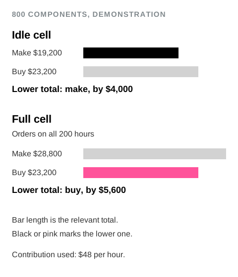
| Relevant total | $19,200 | $23,200 |
Making costs $4,000 less. The allocated $5 per component is $4,000 across 800 units, and it is paid in both columns, so the $4,000 gap is unchanged. Fold that $5 into the make cost and both columns show $29 a component. The gap on the page becomes zero, while the cash gap is still $4,000 in favor of making.
Full cell, with an order for every freed hour
The cell has 200 hours, which is the time the 800 components need. Orders for the other product cover all 200 hours, 200 units. Making every component means those 200 units do not ship.
Opportunity cost = 200 x $48 = $9,600. Per component that is 0.25 x $48 = $12, and 800 x $12 = $9,600.
Scroll horizontally to see all columns.
| Make all 800 | Buy all 800 | |
|---|---|---|
| Avoidable make cost | $19,200 | $0 |
| Purchase-and-delivery | $0 | $23,200 |
| Opportunity cost | $9,600 | $0 |
| Relevant total | $28,800 | $23,200 |
Buying costs $5,600 less. Per component, buying costs $5 more in cash ($29 against $24) and frees $12 of contribution. The net is $7, and 800 x $7 = $5,600.
Substituting the $80 selling price for the $48 contribution changes the full-cell result. Opportunity cost becomes 200 x $80 = $16,000, the make total becomes $35,200, and buying appears to save $12,000. The extra $6,400 is 200 hours x $32 of variable cost the other product would have used. Dropping the order also drops that variable cost, so it is not a benefit you lose. The downtime article linked above is the same distinction, under a stop rather than a component.
Demand ceiling: 80 orders on a full cell
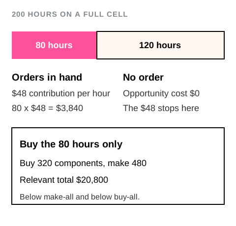
Keep the 200-hour cell. Confirmed orders cover 80 units of the other product, which is 80 hours. The other 120 hours have no order.
Make all 800 components and the opportunity cost is 80 x $48 = $3,840. The relevant total to make is 19,200 + 3,840 = $23,040. The relevant total to buy all 800 is $23,200. Making everything is $160 cheaper than buying everything, on a cell that is already full, because 120 of the 200 hours have nothing to sell.
Buying only the slice that frees those 80 hours is lower still. At 0.25 hour per component, 80 / 0.25 = 320 components bought, and 480 still made. Those 480 use 120 hours. The 80 orders use the other 80. The cell stays full.
Scroll horizontally to see all columns.
| Make 480, buy 320 | Make all 800 | Buy all 800 | |
|---|---|---|---|
| Avoidable make cost | 480 x $24 = $11,520 | $19,200 | $0 |
| Purchase-and-delivery | 320 x $29 = $9,280 | $0 | $23,200 |
| Opportunity cost | $0, the 80 orders still ship | $3,840 | $0 |
| Relevant total | $20,800 | $23,040 | $23,200 |
$20,800 is $2,240 below making everything and $2,400 below buying everything.
The check on the 320 components you switch: each costs $5 more to buy than to make, so 320 x $5 = $1,600 of extra cash. Those 320 free the 80 hours, which keep $3,840 of contribution. $3,840 - $1,600 = $2,240. The other 480 stay in-house. Buying them would add $5 each and would free hours with no order.
Two-scenario decision table
Scroll horizontally to see all columns.
| Idle: 400 hours, and the 80 orders still fit | Full: 200 hours, orders for all 200 | |
|---|---|---|
| Relevant cost to make 800 | $19,200 | $28,800 |
| Relevant cost to buy 800 | $23,200 | $23,200 |
| Lower relevant total | Make, by $4,000 | Buy, by $5,600 |
| Contribution per constrained hour | $48, and none of it is added | $48, added for all 200 hours |
| Demand ceiling used | 80 ordered hours, all still covered | 200 ordered hours, all displaced |
| Unavoidable $5 per component | Flagged, in neither total | Flagged, in neither total |
When the ceiling is 80 hours on that same full cell, the lower total is the partial buy at $20,800. The cell is still full. The orders are shorter than the hours the component uses.
After you replace an input, recompute these checks. Avoidable make cost is the sum of the four changing make lines. Purchase-and-delivery is price plus freight and receiving. Contribution per constrained hour is (price - variable cost) / hours per unit. Opportunity cost is that rate times ordered hours you would actually drop. The partial quantity to buy is ordered hours divided by hours per component.
What the table leaves to you
The lower relevant total is the cost answer for one period and the hours you typed in. A few conditions can override it.
The purchased component has to meet the spec, and it has to arrive in time for the schedule that uses the freed hours. Write the period the quote covers next to the purchase price. A later price is a new purchase-and-delivery cost.
The machines in this comparison are already owned. Depreciation of those machines sits in the unavoidable flag. Buying a packaging line you do not yet have, or sending the packing to a contract packer, is a different cash comparison, in Contract Packing Versus Owning a Packaging Line. That article’s break-even is about equipment you would acquire. It does not price an hour on a cell you already run.
Several products competing for the same hours need their own contribution per constrained hour, each stopped at its own orders. This page answers one question: with one other product that already has orders, is the component cheaper to make or to buy?
The Production Economics guide collects the related plant-cost articles. The editorial policy states how a worked example on this site is labeled. Replace the demonstration before you act on a total.
Methods and sources
Updated October 12, 2026. WonksAnonymous Editors prepared this explanation with AI assistance. No audit of a factory’s books is claimed. Every dollar amount and every hour in the demonstration is an original illustrative input, and the totals above are the products of those inputs. No company is named. The page states no machine model, speed, dimension, power rating, certification, or customer project.
Definitions were read from OpenStax, Principles of Accounting, Volume 2: Managerial Accounting (Mitchell Franklin, Patty Graybeal, and Dixon Cooper; published February 14, 2019; Houston). The text used here was captured on October 11, 2026. The textbook’s own numerical examples are not reused.
- 10.1 Identify Relevant Information for Decision-Making: relevant, avoidable, unavoidable, sunk, and opportunity cost.
- 10.3 Evaluate and Determine Whether to Make or Buy a Component: avoidable manufacturing cost against a purchase price, and the qualitative limits of that comparison.
- 10.6 Evaluate and Determine How to Make Decisions When Resources Are Constrained: contribution margin per unit of the scarce resource, the limit set by unsatisfied demand, and outsourcing as one way to free a bottleneck.
A local research-library query for “make or buy relevant cost” on October 12, 2026 returned unrelated pages, so none of those pages are cited. The arithmetic in the demonstration can be repeated from the input table alone.