 WonksAnonymous

Variable Cost Formula: Packaging Line Examples Across Shift Limits
Model packaging materials, piecework, overtime and energy separately, with assumed examples showing where one variable rate stops working.
Extending one variable cost formula beyond a packaging line’s regular shift can understate the cost of the next run. Calculate direct packaging materials and piecework from their quantities, overtime from hours beyond the scheduled shift, and energy from running consumption plus any additional operating blocks.
The starting model, VC = v × Q, works when the unit rate stays constant; the fixed, variable and total cost formulas explain that case. Here, the task is to replace that constant rate when operating conditions change. OpenStax’s cost-behavior chapter distinguishes proportional, mixed and stepped costs, and ties their behavior to an activity driver and relevant range. The packaging calculations below are original assumed examples, not factory observations or industry benchmarks.
Separate the four drivers before adding them
Use a single day and count packaging attempts, including attempts that later fail inspection. Call that count Q. Counting attempts keeps material consumed on rejects inside the model; saleable output comes later.
The assumed line runs at 600 attempts per hour, with eight regular production hours and at most two overtime hours. There are no changeovers or speed losses in this teaching model. Its valid range is 0–6,000 attempts per day. Actual scheduling needs the line’s bottleneck throughput, rather than nameplate speed.
Scroll horizontally to see all columns.
| Component | Assumed driver and cost input | Dominant Failure Mode & Prevention |
|---|---|---|
| Direct packaging materials | $0.12 per attempt for the consumed pouch, label and allocated case material | Reject consumption disappears if only good packs are counted; reconcile issues and returns against attempts. |
| Piecework finishing labor | $0.03 per attempted pack handled by a separate finishing crew | The same worker is charged by piece and again by hour; identify which payroll group each line covers. |
| Overtime technicians | $45 per crew-hour after eight production hours; proportional billing, with no minimum call-out | One extra pack triggers a different hourly cost regime; use the actual staffing agreement and clocked hours. |
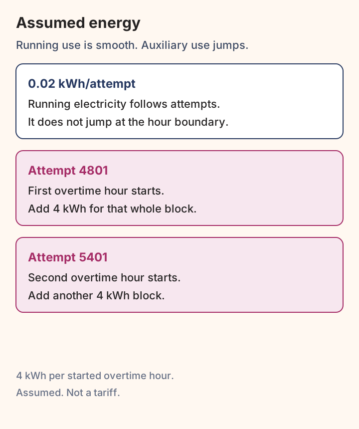
| Running electricity and added auxiliary operation | 0.02 kWh per attempt, plus 4 kWh per started overtime hour; $0.15 per kWh | Metered energy, fixed charges and block operation are blended; separate them before calculating. |
Every value in this table is assumed. The overtime amount is the full added cost of the technician crew for an overtime hour. It is not a premium to add to another hourly wage already included here. Regular technician payroll is treated as committed for the day and sits outside this output-responsive subtotal. The piecework finishers are a different group.
Site rent, regular payroll, standing electricity charges, financing and equipment acquisition are outside this subtotal too. They may matter to a wider decision, but adding them requires a separately labeled scope. These are cost components, not equipment price estimates.
Use a formula that changes after the regular shift
Compute overtime hours first, then apply the overtime rate only to those hours. With r as attempts per hour and H as regular hours:
Overtime hours h(Q) = max(Q / r − H, 0)
Regular-shift limit Qr = r × H
Assumed worked example: Qr = 600 attempts/hour × 8 hours = 4,800 attempts/day; at Q = 5,400, h(Q) = max(5,400 ÷ 600 − 8, 0) = 1 overtime hour.
For this model, let m be material dollars per attempt, p piecework dollars per attempt, e running kWh per attempt, t dollars per kWh, w overtime dollars per crew-hour, and b additional kWh per started overtime hour. Then:
Output-responsive subtotal C(Q)
  = (m + p + e × t) × Q + w × h(Q) + b × t × ceil(h(Q))

Assumed model, Q an integer from 0 to 6,000 attempts/day:
C(Q) = 0.153Q + 0.075 × max(Q − 4,800, 0)
       + 0.60 × ceil(max(Q − 4,800, 0) / 600)
Here ceil rounds up to a whole block; ceil(0) = 0. C is dollars per day. The $0.153 per attempt combines $0.12 materials, $0.03 piecework and $0.003 running electricity. The $0.075 coefficient converts $45 per overtime crew-hour into dollars per attempt at the assumed 600 attempts/hour. None of these is a universal unit rate.
Assumed worked example: C(5,400) = $0.153 × 5,400 + $45 × 1 + 4 kWh × $0.15/kWh × 1 = $871.80/day.
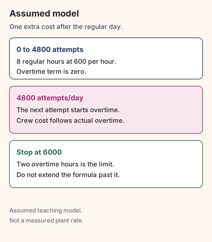
The overtime term creates a change in slope after 4,800 attempts. It does not reprice the first 4,800 attempts. If the real agreement has a minimum overtime payment, replace the proportional-hours term with that payment rule; do not keep this formula unchanged.
Keep an energy step separate from an overtime slope
Running electricity follows attempts here; the auxiliary block jumps when another overtime hour starts. The assumed auxiliary is a separate ventilation or cooling unit activated for an entire one-hour block, consuming 4 kWh per block even when production uses only part of it. This operating rule creates the step; it is not a claim about an electricity tariff.
Scroll horizontally to see all columns.
| Daily attempts, all assumed | Materials | Piecework | Technician overtime | Running + auxiliary electricity | C(Q), rounded |
|---|---|---|---|---|---|
| 4,800 | $576.00 | $144.00 | $0.00 | $14.40 + $0.00 | $734.40 |
| 4,801 | $576.12 | $144.03 | $0.075 | $14.403 + $0.60 | $735.23 |
| 5,400 | $648.00 | $162.00 | $45.00 | $16.20 + $0.60 | $871.80 |
| 6,000 | $720.00 | $180.00 | $90.00 | $18.00 + $1.20 | $1,009.20 |
Retain unrounded values inside the model. At 4,801 attempts, the exact subtotal is $735.228. Relative to 4,800 attempts, that first additional attempt adds $0.828: the ordinary $0.153, $0.075 overtime and a $0.60 auxiliary activation. The next attempt adds $0.228 until another block begins. The second auxiliary block starts at 5,401 attempts.
For the assumed 600-attempt extension from 4,800 to 5,400, incremental cost is ($871.80 − $734.40) ÷ 600 = $0.229 per extra attempt. Multiplying those extra attempts by the regular-range $0.153 would miss $45.60. Use the change in total cost for the additional order, rather than the average of the whole day’s production.
Rules of Thumb for the next production run
Check thresholds against the schedule and records before using a unit rate:
- At Q ≤ 4,800 attempts/day in this assumed model, overtime and auxiliary-block terms are zero. The responsive subtotal is $0.153Q; committed daily costs remain outside it.
- At Q > 4,800, price technician overtime and the first auxiliary block. At Q > 5,400, include a second auxiliary block. These are model thresholds, not recommended factory limits.
- At Q > 6,000, stop: the assumed ten-hour operating window has been exceeded. Obtain another staffing and capacity scenario before extending the calculation.
- At good-pack yield y < 1, divide by Q × y for cost per good pack. At Q × y = 0, a per-good-pack average is undefined.
Assumed denominator example: 5,000 attempts × 0.98 yield = 4,900 good packs; C(5,000) = $780.60, so $780.60 ÷ 4,900 = $0.1593 per good pack for this subtotal. Dividing by attempts would give $0.1561. Do not add the rejected packs’ material cost again: all 5,000 attempts already consumed material in the calculation. Cost per good pack explains the broader operating-cost denominator and double-counting check.
Before budgeting, collect material issues less returns, separate piecework records, technician hours, auxiliary operating intervals and energy readings for the same run. A higher reject rate changes attempts per saleable pack; a changeover changes available hours. Neither should be hidden inside a reused average.
If the question is the cost transferred into finished-goods inventory, move to the cost of goods manufactured formula and WIP reconciliation. That schedule includes manufacturing costs on its chosen accounting basis and adjusts for unfinished work; this daily responsive-cost model does neither. The Production Economics guide connects both calculations to the wider production decision.
Methods and sources
Updated October 2026. WonksAnonymous Editors prepared this AI-assisted analysis. Cost classifications were checked against OpenStax, Principles of Accounting, Volume 2: Managerial Accounting, section 2.2, accessed October 19, 2026. All packaging quantities, payment rules, energy inputs and dollar amounts are original assumed teaching inputs. The arithmetic demonstrates their consequences; it does not establish plant performance, payroll requirements or an industry benchmark.