 WonksAnonymous
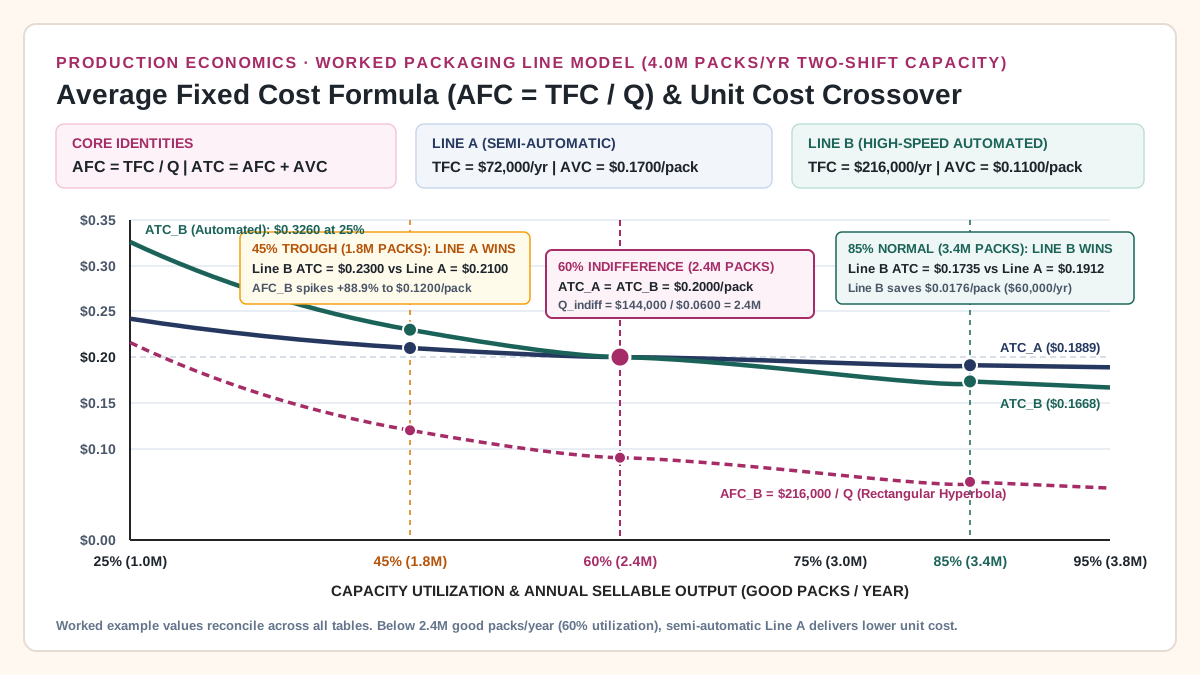
Average Fixed Cost Formula, Cost Per Unit Calculator, and Operating Leverage
Use the average fixed cost formula (AFC = TFC / Q) and unit cost calculator to see why an automated line costs more per pack than a semi-automatic line at 45% utilization.
Updated October 25, 2026. Evaluating a capital-intensive packaging line at a single utilization rate hides how fast fixed overhead inflates unit cost when orders slow down or frequent changeovers cut running hours. The average fixed cost formula divides total period fixed cost by sellable good output (AFC = TFC / Q), forming a rectangular hyperbola where a drop from 85% to 45% capacity utilization increases fixed cost per pack by 88.89% (85 / 45 = 1.8889x) and reverses the unit-cost advantage of high-speed automation.
Use the six identities below before comparing equipment quotes or building a cost per unit calculator. In every equation, Q represents sellable good units completed within the stated accounting period (Q > 0).
Scroll horizontally to see all columns.
| Metric | Exact Algebraic Formula | Mathematical Geometry & Elasticity | Operational Scope & Boundary |
|---|---|---|---|
Average Fixed Cost (AFC) |
AFC = TFC / Q = ATC - AVC |
Rectangular hyperbola (AFC × Q = TFC = constant inside the relevant range); output elasticity of AFC is -1.00. |
TFC covers straight-line equipment depreciation, allocated floor space, insurance, property taxes, and committed preventive maintenance contracts. |
Effective Average Variable Cost (AVC) |
AVC = TVC / Q = AVC_nom / (1 - Scrap_Rate) |
Constant per good unit inside a single shift’s linear operating window; steps up when overtime crew rates or auxiliary energy blocks engage. | Covers rollstock film or pouches, labels, corrugated cases, direct operator wages not committed as fixed overhead, variable servo power, and scrap allowance. |
Average Total Cost Per Unit (ATC) |
ATC = TC / Q = (TFC + TVC) / Q = AFC + AVC |
L-shaped curve within the two-shift relevant range: asymptotically approaches AVC as Q expands and diverges toward infinity as Q approaches zero. |
Primary output when learning how to calculate average cost per unit. Period TFC must be divided by Q before adding unit AVC. |
Cost Indifference Volume (Q_indiff) |
Q_indiff = (TFC_B - TFC_A) / (AVC_A - AVC_B) |
Unique annual good-pack volume where ATC_A = ATC_B and TC_A = TC_B. |
Below Q_indiff, lower-fixed-cost Line A wins; above Q_indiff, lower-variable-cost Line B wins. |
Degree of Operating Leverage (DOL) |
DOL = Contribution_Margin / EBIT = 1 + (TFC / EBIT) |
Dimensionless multiplier at output Q where %ΔEBIT = DOL × %ΔQ. |
Higher TFC raises DOL, magnifying operating income gains above crossover and magnifying profit compression during demand troughs. |
Unallocated Fixed Overhead (GAAP / IAS 2) |
Unallocated_OH = max(0, TFC × (1 - Q_actual / Q_normal)) |
Linear period expense charge whenever actual good output Q_actual falls below normal capacity Q_normal. |
Under US GAAP ASC 330-10-30 and IAS 2.13, idle-capacity fixed overhead cannot be capitalized into ending inventory and must be expensed in current-period COGS. |
Average fixed cost formula and how to calculate average cost per unit
In short-run production economics, total production cost splits into obligations that remain fixed for the time period and input expenses that scale with throughput. As formalized in OpenStax Principles of Economics 3e, Section 7.3 (Costs in the Short Run), total cost (TC) is the sum of total fixed cost (TFC) and total variable cost (TVC):
TC = TFC + TVC
AFC = TFC / Q
AVC = TVC / Q
ATC = TC / Q = (TFC / Q) + (TVC / Q) = AFC + AVC
When an engineering or finance team asks how to calculate average cost per unit, the calculation requires two reconciliations before any division takes place. First, every dollar in TFC and TVC must belong to the same calendar window—whether one month, one quarter, or one 250-day operating year—as detailed in Fixed, Variable and Total Cost Formulas. Second, the denominator Q must count sellable good units that pass inspection, never theoretical machine cycles or raw packaging attempts.
As Vorne Industries’ Calculating OEE (Availability × Performance × Quality) and our Overall Equipment Effectiveness Formula, Calculator, and the OEE Financial Bridge establish, line losses erode output through three multiplicative factors: unplanned and changeover stops reduce Availability, micro-stops and reduced cycle speeds lower Performance, and startup or seal rejects reduce Quality. Because rejected packages consume film, pouches, labels, and variable energy before failing inspection, nominal variable cost per machine cycle (AVC_nom) must be divided by the OEE Quality yield (1 - Scrap_Rate) to express effective variable cost per good pack (AVC_eff), a rule derived step by step in Cost per Good Pack:
Q_good = Q_attempts × (1 - Scrap_Rate)
AVC_eff = AVC_nom / (1 - Scrap_Rate)
Rectangular hyperbola geometry and unit output elasticity (-1)
Unlike unit variable cost, which remains constant across the linear relevant range defined in OpenStax Principles of Managerial Accounting, Section 2.2 (Cost Behavior Patterns), average fixed cost (AFC = TFC / Q) traces a rectangular hyperbola. At any output Q within the staffing and facility relevant range, the product of average fixed cost and quantity equals the constant period overhead (AFC × Q = TFC).
Differentiating AFC = TFC × Q^(-1) with respect to Q yields the point output elasticity of average fixed cost:
e_AFC,Q = (dAFC / dQ) × (Q / AFC) = (-TFC / Q^2) × (Q / (TFC / Q)) = -1.00
For large discrete utilization shifts from an initial utilization U_1 to a lower utilization U_2 while TFC stays constant, the exact ratio of the new average fixed cost (AFC_2) to the initial average fixed cost (AFC_1) is the inverse ratio of capacity utilization:
AFC_2 / AFC_1 = (TFC / Q_2) / (TFC / Q_1) = Q_1 / Q_2 = U_1 / U_2
When a packaging line drops from 85% normal two-shift utilization to 45% single-shift trough utilization, AFC does not rise by 40%; it multiplies by 85 / 45 = 1.8889, an +88.89% spike in fixed cost on every pack produced.
Takeaway: Average fixed cost (AFC = TFC / Q) is inversely proportional to sellable output; halving utilization doubles the fixed overhead burden carried by every good unit.
Cost per unit calculator: automated vs semi-automatic packaging lines
To see how AFC and AVC interact in capital budgeting, consider a plant evaluating two machinery configurations for a pouch-and-carton line with a theoretical two-shift capacity (Q_max) of 4,000,000 good packs/year (250 operating days × 2 shifts/day × 8 scheduled hours/shift = 4,000 hours/year at an effective two-shift ceiling of 1,000 good packs/hour). Each good pack carries an internal transfer credit or contract selling price (P) of $0.2500/pack ($250.00 per 1,000 good packs).
Worked example. Replace each input with a quote or a measured figure from the plant before using the result.
- Line A (Semi-Automatic Packaging Line): Installed capital expenditure is
$160,000with a$10,000salvage value over a5-yearstraight-line life ($30,000/yearannual equipment charge), plus$42,000/yearin allocated floor space, property insurance, preventive maintenance, and line supervision, givingTFC_A = $72,000/year. Variable cost isAVC_A = $0.1700/good pack($0.0900packaging film and carton materials including a2.0%scrap allowance,$0.0750direct operator labor, and$0.0050variable energy). - Line B (High-Speed Automated Packaging Line): Installed capital expenditure is
$1,050,000with a$70,000salvage value over a7-yearstraight-line life ($140,000/yearannual equipment charge), plus$76,000/yearin floor space, OEM service contract, insurance, and dedicated automation technician coverage, givingTFC_B = $216,000/year(3.0xLine A’s fixed overhead). Automation cuts tending labor and film waste, lowering variable cost toAVC_B = $0.1100/good pack($0.0850rollstock film and case material including a1.5%scrap allowance,$0.0180tending operator labor, and$0.0070servo power and compressed air).
Copyable spreadsheet cost per unit calculator (B2:C15)
Build this two-column calculator in Excel or Google Sheets to evaluate both lines at any annual volume Q. Enter raw numbers without currency formatting in rows 2 through 7; rows 8 through 15 compute totals, unit averages, indifference volume, break-even thresholds, and operating leverage automatically. For multi-stage manual, semi-automatic, and automatic comparisons across wider shift limits, pair this layout with the Manual, Semi-Automatic or Fully Automatic Packaging Cost Model and Variable Cost Formula: Packaging Line Examples Across Shift Limits.
Scroll horizontally to see all columns.
| Row | Metric / Calculator Line | Col B: Line A (Semi-Auto) Input or Formula | Col C: Line B (Automated) Input or Formula | Value at 85% (3.4M Packs) |
Value at 45% (1.8M Packs) |
|---|---|---|---|---|---|
| 2 | Two-shift capacity Q_max (packs/yr) |
4000000 |
4000000 |
4,000,000 |
4,000,000 |
| 3 | Period good output Q (packs/yr) |
3400000 |
=B3 |
3,400,000 |
1,800,000 |
| 4 | Capacity utilization U (%) |
=B3/B2 |
=C3/C2 |
85.00% |
45.00% |
| 5 | Annual Fixed Cost TFC ($/yr) |
72000 |
216000 |
$72,000 vs $216,000 |
$72,000 vs $216,000 |
| 6 | Effective Variable Cost AVC ($/pack) |
0.1700 |
0.1100 |
$0.1700 vs $0.1100 |
$0.1700 vs $0.1100 |
| 7 | Selling / Transfer Price P ($/pack) |
0.2500 |
0.2500 |
$0.2500 |
$0.2500 |
| 8 | Average Fixed Cost AFC ($/pack) |
=IF(B3>0, B5/B3, NA()) |
=IF(C3>0, C5/C3, NA()) |
$0.0212 vs $0.0635 |
$0.0400 vs $0.1200 |
| 9 | Average Total Cost ATC ($/pack) |
=B8+B6 |
=C8+C6 |
$0.1912 vs $0.1735 |
$0.2100 vs $0.2300 |
| 10 | Cost per 1,000 good packs ($/1,000) |
=B9*1000 |
=C9*1000 |
$191.18 vs $173.53 |
$210.00 vs $230.00 |
| 11 | Total Annual Cost TC ($/yr) |
=B5+(B6*B3) |
=C5+(C6*C3) |
$650,000 vs $590,000 |
$378,000 vs $414,000 |
| 12 | Unit Contribution Margin CM ($/pack) |
=B7-B6 |
=C7-C6 |
$0.0800 vs $0.1400 |
$0.0800 vs $0.1400 |
| 13 | Break-Even Volume Q_BE (packs/yr) |
=B5/B12 |
=C5/C12 |
900,000 vs 1,542,857 |
900,000 vs 1,542,857 |
| 14 | Annual Operating Profit EBIT ($/yr) |
=(B12*B3)-B5 |
=(C12*C3)-C5 |
$200,000 vs $260,000 |
$72,000 vs $36,000 |
| 15 | Degree of Operating Leverage DOL |
=(B12*B3)/B14 |
=(C12*C3)/C14 |
1.36x vs 1.83x |
2.00x vs 7.00x |
Deriving the break-even and cost indifference crossover volumes
Following OpenStax Principles of Managerial Accounting, Section 3.2 (Break-Even Point in Units and Dollars), a line reaches its break-even volume (Q_BE) where total contribution margin equals total fixed cost (Q_BE × (P - AVC) = TFC):
Q_BE_A = $72,000 / ($0.2500 - $0.1700) = $72,000 / $0.0800 = 900,000 good packs/year (22.50% utilization)
Q_BE_B = $216,000 / ($0.2500 - $0.1100) = $216,000 / $0.1400 = 1,542,857 good packs/year (38.57% utilization)
Because Line B carries $144,000/year more fixed overhead than Line A ($216,000 - $72,000) while saving $0.0600/pack in variable cost ($0.1700 - $0.1100), setting ATC_A = ATC_B identifies the exact Cost Indifference Volume (Q_indiff):
(TFC_A / Q_indiff) + AVC_A = (TFC_B / Q_indiff) + AVC_B
Q_indiff = (TFC_B - TFC_A) / (AVC_A - AVC_B)
Q_indiff = ($216,000 - $72,000) / ($0.1700 - $0.1100) = $144,000 / $0.0600 = 2,400,000 good packs/year (60.00% utilization)
At Q_indiff = 2,400,000 good packs/year, both lines incur the exact same total annual cost ($480,000/year) and the exact same average total cost per unit ($0.2000/pack, or $200.00 per 1,000 packs):
- Line A at
2.4Mpacks:AFC_A = $72,000 / 2,400,000 = $0.0300/pack;ATC_A = $0.0300 + $0.1700 = $0.2000/pack. - Line B at
2.4Mpacks:AFC_B = $216,000 / 2,400,000 = $0.0900/pack;ATC_B = $0.0900 + $0.1100 = $0.2000/pack.
Takeaway: Automation only lowers unit cost when sustained good output exceeds Q_indiff = (TFC_B - TFC_A) / (AVC_A - AVC_B); below 2,400,000 good packs/year (60% utilization), the semi-automatic line is cheaper per pack.
Why dropping from 85% to 45% utilization flips the unit-cost winner
Equipment proposals routinely benchmark automated machinery at 85% capacity utilization (3,400,000 good packs/year across two shifts). As the Federal Reserve Board explains in its Industrial Production and Capacity Utilization (G.17) Explanatory Notes, sustainable practical capacity reflects realistic work schedules and normal maintenance downtime rather than uninterrupted nameplate speed. On the plant floor, however, seasonal demand troughs, single-shift staffing, or fragmented multi-SKU changeover schedules regularly pull actual annual output down to 45% of two-shift capacity (1,800,000 good packs/year). Look at Manufacturing Capacity Utilization: Macro Index vs Plant Floor and How Equipment Utilization Changes Automation Payback for how denominator shifts alter payback horizons.
The table below tracks AFC, AVC, ATC, total cost (TC), annual operating profit (EBIT), and DOL across six utilization tiers from 25% (1.0M packs) to 95% (3.8M packs).
Worked example. Replace each input with a quote or a measured figure from the plant before using the result.
Scroll horizontally to see all columns.
Capacity Utilization (% of 4.0M) |
Annual Good Packs (Q) |
Line A AFC_A ($/pack) |
Line A ATC_A ($/pack) |
Line A Annual TC_A |
Line A EBIT_A (DOL_A) |
Line B AFC_B ($/pack) |
Line B ATC_B ($/pack) |
Line B Annual TC_B |
Line B EBIT_B (DOL_B) |
Unit-Cost Winner & Annual Savings |
|---|---|---|---|---|---|---|---|---|---|---|
25% (Single-Shift Low) |
1,000,000 |
$0.0720 |
$0.2420 |
$242,000 |
$8,000 (10.00x) |
$0.2160 |
$0.3260 |
$326,000 |
-$76,000 (-1.84x) |
Line A (Semi-Auto) by $0.0840/pack ($84,000/yr) |
45% (Demand Trough) |
1,800,000 |
$0.0400 |
$0.2100 |
$378,000 |
$72,000 (2.00x) |
$0.1200 |
$0.2300 |
$414,000 |
$36,000 (7.00x) |
Line A (Semi-Auto) by $0.0200/pack ($36,000/yr) |
60% (Q_indiff Crossover) |
2,400,000 |
$0.0300 |
$0.2000 |
$480,000 |
$120,000 (1.60x) |
$0.0900 |
$0.2000 |
$480,000 |
$120,000 (2.80x) |
Exact Tie at $0.2000/pack ($480,000/yr) |
75% (Two-Shift Moderate) |
3,000,000 |
$0.0240 |
$0.1940 |
$582,000 |
$168,000 (1.43x) |
$0.0720 |
$0.1820 |
$546,000 |
$204,000 (2.06x) |
Line B (Automated) by $0.0120/pack ($36,000/yr) |
85% (Normal Capacity) |
3,400,000 |
$0.0212 |
$0.1912 |
$650,000 |
$200,000 (1.36x) |
$0.0635 |
$0.1735 |
$590,000 |
$260,000 (1.83x) |
Line B (Automated) by $0.0176/pack ($60,000/yr) |
95% (Peak Schedule) |
3,800,000 |
$0.0189 |
$0.1889 |
$718,000 |
$232,000 (1.31x) |
$0.0568 |
$0.1668 |
$634,000 |
$316,000 (1.68x) |
Line B (Automated) by $0.0221/pack ($84,000/yr) |
Step-by-step arithmetic of the 85% vs 45% reversal
- At
85%normal two-shift utilization (Q = 3,400,000good packs/year):- Line B (Automated) spreads its
$216,000fixed overhead down toAFC_B = $216,000 / 3,400,000 = $0.063529/pack. AddingAVC_B = $0.1100/packgivesATC_B = $0.1735/pack($173.53 per 1,000 packs, or$590,000/yeartotal cost). - Line A (Semi-Automatic) has
AFC_A = $72,000 / 3,400,000 = $0.021176/pack. AddingAVC_A = $0.1700/packgivesATC_A = $0.1912/pack($191.18 per 1,000 packs, or$650,000/yeartotal cost). - Result at
85%: Automated Line B wins by$0.0176/pack($17.65 per 1,000 packs), saving$60,000/year.
- Line B (Automated) spreads its
- When utilization drops to
45%(Q = 1,800,000good packs/year):- Both lines suffer an
+88.89%increase inAFC(3,400,000 / 1,800,000 = 1.8889x), but the dollar impact scales withTFC. - On Line A,
AFC_Arises by only+$0.0188/pack(from$0.0212to$0.0400/pack), liftingATC_Ato$0.2100/pack($378,000/year). - On Line B,
AFC_Bjumps by+$0.0565/pack(from$0.0635to$0.1200/pack). Because that+$0.0565/packfixed-cost penalty exceeds Line B’s$0.0600/packvariable-cost advantage over the remaining volume below2.4M,ATC_Bclimbs to$0.2300/pack($414,000/year). - Result at
45%: Semi-automatic Line A beats automated Line B by$0.0200/pack($20.00 per 1,000 packs), saving$36,000/year.
- Both lines suffer an
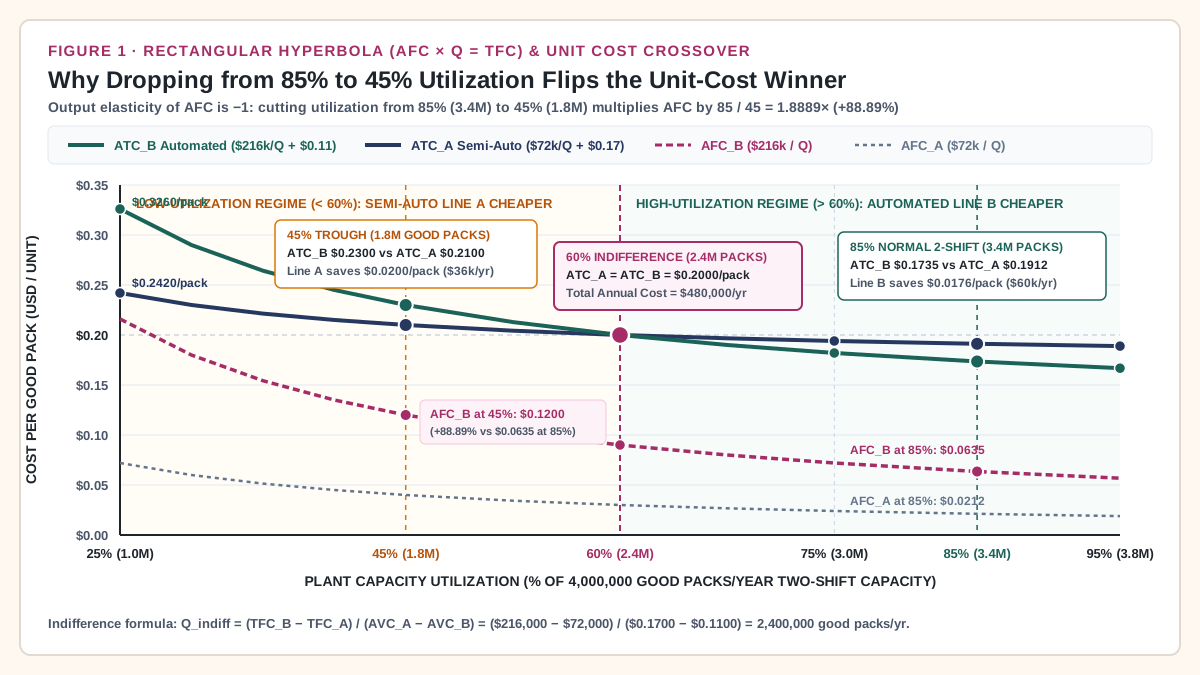
Takeaway: A +88.89% spike in AFC between 85% and 45% utilization adds $0.0565/pack to the automated line but only $0.0188/pack to the semi-automatic line, flipping a $60,000/year automation savings into a $36,000/year cost penalty.
Degree of operating leverage (DOL) when volume drops
The unit-cost reversal is the mirror image of operating leverage. As defined in OpenStax Principles of Managerial Accounting, Section 3.5 (Margin of Safety and Operating Leverage), the Degree of Operating Leverage (DOL) at a given output Q is the ratio of total contribution margin to net operating income (EBIT):
Contribution_Margin = Q × (P - AVC)
EBIT = Q × (P - AVC) - TFC = Contribution_Margin - TFC
DOL = Contribution_Margin / EBIT = 1 + (TFC / EBIT)
DOL measures the exact elasticity of operating profit with respect to output volume (%ΔEBIT = DOL × %ΔQ). Notice how DOL = 1 + (TFC / EBIT) links directly to the average fixed cost formula: dividing both numerator and denominator of TFC / EBIT by Q yields:
DOL = 1 + [ AFC / (P - ATC) ]
Whenever utilization drops, AFC rises and unit operating margin (P - ATC) shrinks, causing DOL to climb hyperbolically as output approaches the break-even threshold Q_BE.
Quantifying profit compression between 85% and 45% utilization
Compare both packaging lines when annual good output falls by -47.0588% (-1,600,000 packs, from 3,400,000 packs at 85% utilization to 1,800,000 packs at 45% utilization):
- At
85%utilization (3,400,000good packs):- Line A (Semi-Auto): Contribution margin is
3,400,000 × $0.0800 = $272,000. SubtractingTFC_A = $72,000yieldsEBIT_A = $200,000andDOL_A = $272,000 / $200,000 = 1.36x. - Line B (Automated): Contribution margin is
3,400,000 × $0.1400 = $476,000. SubtractingTFC_B = $216,000yieldsEBIT_B = $260,000andDOL_B = $476,000 / $260,000 = 1.8308x.
- Line A (Semi-Auto): Contribution margin is
- Impact of the
-47.0588%volume drop to45%utilization (1,800,000good packs):- Line A EBIT drop:
%ΔEBIT_A = -47.0588% × 1.36 = -64.00%. Operating profit declines from$200,000to$72,000(1,800,000 × $0.0800 - $72,000). At45%utilization,DOL_Arises modestly to$144,000 / $72,000 = 2.00x. - Line B EBIT drop:
%ΔEBIT_B = -47.0588% × 1.8308 = -86.15%. Operating profit plunges from$260,000to$36,000(1,800,000 × $0.1400 - $216,000)—half of Line A’s profit at the same trough volume. Worse, at45%utilization, Line B’s operating leverage reachesDOL_B = $252,000 / $36,000 = 7.00x, meaning every additional10%drop in pack volume wipes out70%of remaining operating income.
- Line A EBIT drop:
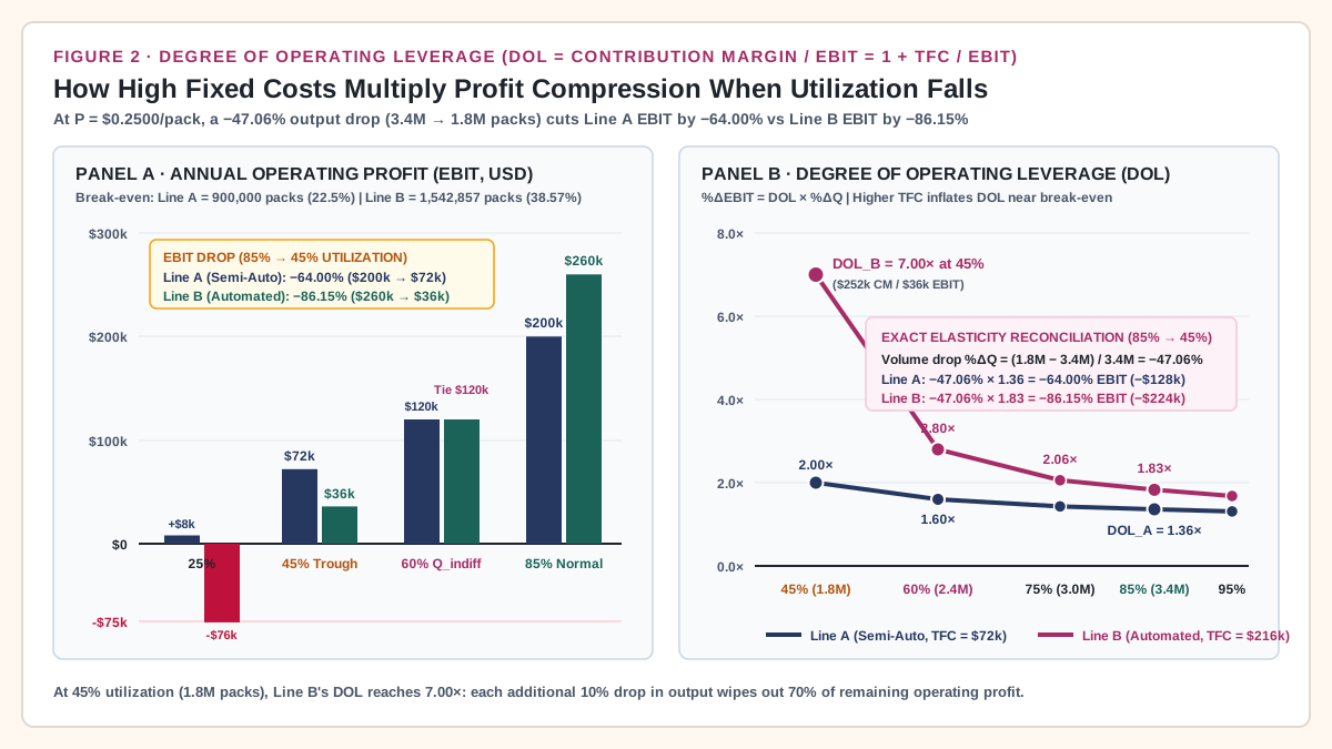
Takeaway: High fixed overhead raises both the break-even floor (38.57% vs 22.50%) and the DOL multiplier, turning a 47.06% volume pullback into an 86.15% operating profit collapse on the automated line.
Normal capacity vs actual output: why GAAP and IAS 2 forbid inventorying idle fixed cost
When utilization falls to 45% and actual managerial ATC_B rises from $0.1735/pack to $0.2300/pack, a common accounting error is to value ending finished-goods inventory at $0.2300/pack. As shown in OpenStax Principles of Managerial Accounting, Section 6.5 (Variable and Absorption Costing), unrestricted full absorption allows a plant to defer period fixed overhead into unsold inventory on the balance sheet.
To prevent underutilized factories from capitalizing idle machine depreciation as an asset, financial reporting standards and U.S. tax regulations enforce a strict normal capacity ceiling:
- IFRS (
IAS 2 Inventories, Paragraph 13): As published by the IFRS Foundation in IAS 2 Inventories, the allocation of fixed production overheads to the costs of conversion must be based on the normal capacity of the production facilities—defined as the production expected to be achieved on average over a number of periods or seasons under normal circumstances, taking into account the loss of capacity resulting from planned maintenance. Paragraph 13 explicitly mandates that the amount of fixed overhead allocated to each unit of production is not increased as a consequence of low production or idle plant, and that unallocated overheads are recognized as an expense in the period in which they are incurred. - US GAAP (
FASB ASC 330-10-30-3through30-7): MirrorsIAS 2.13word for word, requiring fixed production overhead to be absorbed based on normal capacity and charging abnormally low production variances directly to current-period Cost of Goods Sold (COGS). - U.S. Treasury Inventory Regulations (
26 CFR § 1.471-11): Under the full absorption method and practical capacity provisions of26 CFR § 1.471-11(d)(4), fixed indirect production costs (machinery depreciation, factory rent, property taxes, supervisory salaries) are assigned to units produced using the practical capacity rate, while the cost of idle excess capacity is deducted in the current year.
Reconciling managerial ATC ($0.2300) vs GAAP/IFRS inventoriable unit cost ($0.1735) at 45% utilization
Using Line B’s two-shift steady-state output (Q_normal = 3,400,000 good packs/year at 85% utilization) as the plant’s normal capacity baseline, the standard fixed overhead absorption rate is fixed at $0.063529/pack ($216,000 / 3,400,000). See Cost of Goods Manufactured Formula: A Packaging WIP Reconciliation and Allocate Manufacturing Overhead After Automation for how absorbed overhead flows through work-in-process (WIP) and finished goods.
Worked example. Replace each input with a quote or a measured figure from the plant before using the result.
Scroll horizontally to see all columns.
Accounting & Cost Metric for Automated Line B (TFC_B = $216,000/yr) |
At 85% Normal Capacity (Q = 3,400,000 Packs) |
At 45% Trough Utilization (Q = 1,800,000 Packs) |
Accounting Rule & Reconciliation Formula |
|---|---|---|---|
1. Standard Fixed Overhead Rate (AFC_normal) |
$0.063529 / pack |
$0.063529 / pack |
TFC_B / Q_normal = $216,000 / 3,400,000 (capped under ASC 330-10-30 / IAS 2.13) |
2. Effective Unit Variable Cost (AVC_B) |
$0.110000 / pack |
$0.110000 / pack |
Direct materials (incl. 1.5% scrap), tending labor, and variable servo power |
| 3. GAAP / IFRS Inventoriable Unit Cost | $0.173529 / pack |
$0.173529 / pack |
AFC_normal + AVC_B (maximum unit value permitted on the balance sheet) |
4. Actual Managerial AFC_actual (TFC_B / Q_actual) |
$0.063529 / pack |
$0.120000 / pack |
$216,000 / 1,800,000 = $0.1200/pack (+88.89% managerial fixed-cost spike) |
5. Full Managerial Unit Cost (ATC_actual) |
$0.173529 / pack |
$0.230000 / pack |
AFC_actual + AVC_B = $0.1200 + $0.1100 (true economic burden per pack produced) |
| 6. Unabsorbed Idle Fixed Cost Per Pack | $0.000000 / pack |
$0.056471 / pack |
ATC_actual - Inventoriable_Cost = $0.230000 - $0.173529 |
| 7. Total Fixed Overhead Capitalized to Inventory | $216,000.00 (100.00%) |
$114,352.94 (52.94%) |
Q_actual × AFC_normal = 1,800,000 × $0.06352941 |
8. Unallocated Fixed Overhead Expensed to Period COGS |
$0.00 (0.00%) |
$101,647.06 (47.06%) |
TFC_B × (1 - Q_actual / Q_normal) = $216,000 - $114,352.94 |
At 45% utilization (1,800,000 packs), only $114,352.94 (52.94% of the $216,000 fixed overhead pool) can be attached to inventory. The remaining $101,647.06 (47.06%, representing the 1,600,000 unproduced packs below normal capacity multiplied by $0.06352941/pack) hits the current period’s income statement immediately as an unfavorable production-volume variance inside COGS.
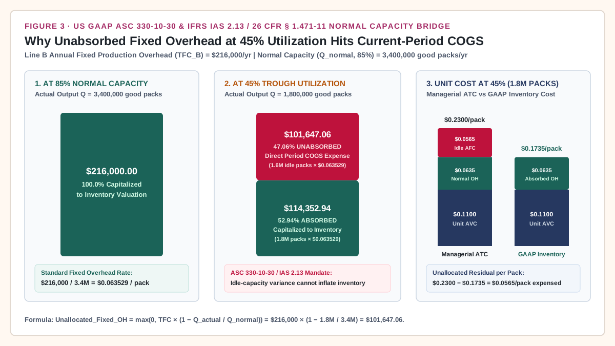
Takeaway: Managerial ATC ($0.2300/pack at 45% utilization) governs pricing and equipment selection, while GAAP/IFRS normal-capacity absorption caps balance-sheet inventory at $0.1735/pack and forces the $101,647.06 idle-capacity penalty straight into current-period COGS.
Common mistakes when applying the average fixed cost formula
Before signing a capital expenditure request or updating standard product costs, audit the model against these five high-frequency engineering and financial failure modes:
Scroll horizontally to see all columns.
| Failure Mode | Root Cause in Plant Models | Financial or Operational Distortion | Engineering & Accounting Prevention Rule |
|---|---|---|---|
1. Using nameplate cycle speed in the AFC denominator |
Dividing TFC by Cycles_per_minute × 60 × Scheduled_Hours without deducting changeover stops, micro-stops, or quality rejects. |
Understates AFC by 25%–55%, making high-fixed-cost automation appear to pay back months earlier than achievable throughput allows. |
Always compute Q = Nameplate_Rate × Scheduled_Hours × Availability × Performance × Quality so only sellable good packs enter AFC = TFC / Q. |
2. Extrapolating constant TFC across step-cost boundaries |
Treating TFC as flat when volume expands past a single-shift or two-shift ceiling (4,000,000 packs/yr in the worked model). |
Ignores the stepped fixed cost jump required for third-shift supervision, added quality inspectors, or a second packaging unit. | Lock each AFC curve to its explicit relevant range (0 < Q ≤ Q_max) and insert a discrete step in TFC wherever a shift or machine threshold is crossed. |
| 3. Counting sunk depreciation as short-run cash savings | Assuming that shutting down an automated line for one shift saves $0.0635/pack in fixed depreciation. |
Confuses committed period depreciation and multi-year lease obligations with avoidable short-run cash outlays. | Separate committed sunk fixed costs (depreciation, property tax) from discretionary or shift-avoidable fixed costs before pricing short-run make-or-buy decisions. |
4. Capitalizing low-utilization AFC spikes into ending inventory |
Recomputing standard inventory overhead rates downward during a 45% demand trough ($0.1200/pack fixed overhead instead of $0.0635/pack). |
Violates ASC 330-10-30 and IAS 2.13 by hiding $101,647.06 of idle plant expense on the balance sheet and overstating operating income. |
Lock inventory overhead absorption to multi-period normal capacity (Q_normal) and expense max(0, TFC × (1 - Q_actual / Q_normal)) in current-period COGS. |
5. Applying a static DOL multiplier across wide volume swings |
Using the 85% utilization DOL (1.83x) to estimate profit sensitivity after volume has already fallen near 45% utilization. |
Misses the non-linear convexity of DOL = 1 + TFC / EBIT, which jumps from 1.83x at 85% utilization to 7.00x at 45% utilization. |
Recompute DOL at each utilization tier in the sensitivity matrix rather than treating operating leverage as a fixed constant. |
Engineering rules of thumb for packaging line selection
- Rule of Thumb 1 (Indifference Buffer): If forecasted minimum seasonal utilization falls below
1.25 × Q_indiff(in our worked model,1.25 × 2.4M = 3.0Mgood packs/year or75%utilization), require modular or semi-automatic equipment options in the bid package so a single-shift demand trough does not push unit cost above semi-automatic levels. - Rule of Thumb 2 (Operating Leverage Ceiling): If
DOL = 1 + (TFC / EBIT)exceeds3.00xat the plant’s conservative volume case, fixed overhead is consuming more than66.7%of contribution margin (TFC / CM > 2/3); reduce committed fixed cost (for example, via contract packing or lower-CapEx semi-automatic cells) before committing capital. - Rule of Thumb 3 (Scrap-Adjusted Variable Cost): Whenever automated rollstock equipment runs higher startup film waste during frequent short-batch changeovers, recalculate
AVC_eff = AVC_nom / (1 - Scrap_Rate)for each batch size before computingQ_indiff.
Return to the Production Economics reading guide to connect fixed-cost spreading with bottleneck throughput, batch changeover sizing, and factory capacity utilization.
Frequently Asked Questions
What is the average fixed cost formula and how does it relate to average total cost?
The average fixed cost formula is AFC = TFC / Q, where TFC is total fixed cost for the accounting period and Q is the count of sellable good units produced in that same period. Because total cost equals fixed cost plus variable cost (TC = TFC + TVC), dividing every term by Q gives ATC = AFC + AVC, which means average fixed cost can also be calculated by subtracting average variable cost from average total cost (AFC = ATC - AVC).
Why does average fixed cost increase by 88.89% when capacity utilization drops from 85% to 45%?
Because total fixed cost (TFC) remains constant inside the relevant range, AFC = TFC / Q forms a rectangular hyperbola (AFC × Q = TFC) with an output elasticity of -1.00. When utilization drops from 85% (3,400,000 packs) to 45% (1,800,000 packs), the ratio of the new average fixed cost to the original average fixed cost is the inverse of the utilization ratio: 85 / 45 = 1.8889, or an +88.89% increase (rising from $0.0635/pack to $0.1200/pack on Automated Line B).
How do you calculate the cost indifference volume between an automated line and a semi-automatic line?
Set the average total cost formulas of the two lines equal (TFC_A / Q + AVC_A = TFC_B / Q + AVC_B) and solve for Q: Q_indiff = (TFC_B - TFC_A) / (AVC_A - AVC_B). In the worked packaging comparison (TFC_A = $72,000, AVC_A = $0.1700/pack; TFC_B = $216,000, AVC_B = $0.1100/pack), Q_indiff = ($216,000 - $72,000) / ($0.1700 - $0.1100) = $144,000 / $0.0600 = 2,400,000 good packs/year (60% capacity utilization), where both lines cost exactly $0.2000/pack.
Can a manufacturer capitalize higher average fixed costs into inventory when utilization drops?
No. Both US GAAP (FASB ASC 330-10-30-3 through 30-7) and IFRS (IAS 2 Inventories, Paragraph 13), along with U.S. tax regulations (26 CFR § 1.471-11), require fixed production overhead to be allocated to inventory based on normal capacity (85% or 3,400,000 packs/year in the worked model, equal to $0.063529/pack). When actual production falls to 45% (1,800,000 packs), only $114,352.94 (52.94%) is capitalized into inventory at $0.063529/pack, while the remaining $101,647.06 (47.06%) of unabsorbed fixed overhead must be expensed immediately in current-period Cost of Goods Sold (COGS).