 WonksAnonymous
Overall Equipment Effectiveness Formula, Calculator, and the OEE Financial Bridge
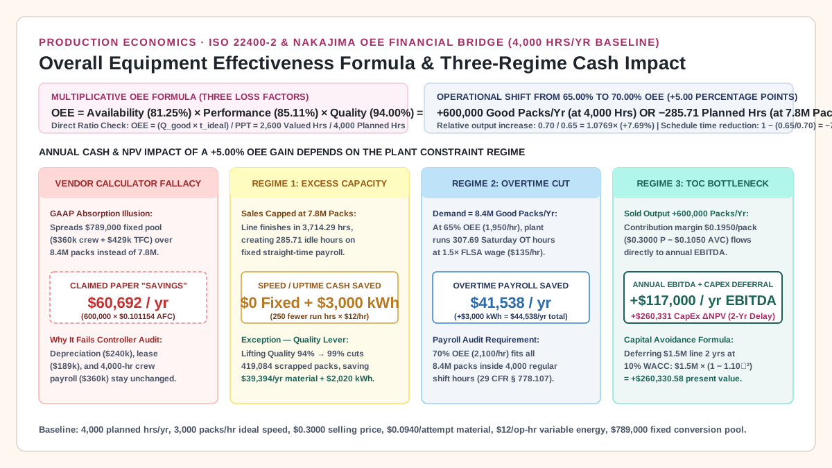
Use the overall equipment effectiveness formula (OEE = Availability × Performance × Quality) and financial calculator to test whether a +5% OEE gain saves cash or merely creates idle time.
Updated October 25, 2026. Multiplying freed machine hours by a full absorption overhead rate causes equipment ROI models to fail controller review whenever straight-time labor and depreciation stay fixed on the income statement.
The overall equipment effectiveness formula (OEE = Availability × Performance × Quality) reduces algebraically to the ratio of valued operating time to planned production time (OEE = (Q_good × t_ideal) / PPT), where unplanned downtime, speed losses, and scrap rejects compound multiplicatively. While raising a 4,000-hour, 3,000-pack/hour packaging line from 65.00% to 70.00% OEE always unlocks +600,000 good packs per year or frees 285.71 planned hours, the real annual cash impact ranges from $0 in fixed-cost savings ($3,000 in variable energy) under excess capacity, to $41,538 in eliminated overtime payroll ($44,538 with energy), to +$117,000 in bottleneck EBITDA plus +$260,331 in present-value CapEx deferral (2-year delay on a $1.5M line at 10% WACC)—unless the gain comes from Quality yield (94% to 99%), which saves $39,394/year in raw material and film scrap across every regime.
Use the six operational and financial identities below before building an overall equipment effectiveness calculator or signing a capital request. In every equation, Q_good counts first-pass sellable units that pass inspection, Q_total counts total attempted machine cycles, and t_ideal is the ideal cycle time (1 / R_ideal).
Scroll horizontally to see all columns.
| Metric & Standard Reference | Exact Algebraic Formula | Algebraic Reduction & Dimension | Operational & Financial Boundary |
|---|---|---|---|
1. Multiplicative OEE (ISO 22400-2 / Nakajima) |
OEE = Availability × Performance × Quality = (T_run / PPT) × ((Q_total × t_ideal) / T_run) × (Q_good / Q_total) |
T_run and Q_total cancel to yield the Direct Ratio Check: OEE = (Q_good × t_ideal) / PPT = T_valued / PPT. |
Measured strictly inside Planned Production Time (PPT); excludes unscheduled shifts, holidays, and planned preventive maintenance shutdowns. |
2. Total Effective Equipment Performance (TEEP) |
TEEP = Utilization × OEE = (PPT / T_cal) × OEE = (Q_good × t_ideal) / 8,760 hrs |
Relates valued productive time (T_valued) to all calendar hours (T_cal = 365 × 24 = 8,760 hrs/yr). |
Quantifies hidden schedule capacity (nights and weekends) before approving capital expenditure for a parallel machine. |
3. Freed Planned Hours at Fixed Demand (Q_bar) |
PPT_req(OEE) = Q_bar / (R_ideal × OEE) and ΔPPT_saved = PPT_0 × (1 - OEE_0 / OEE_1) |
Raising OEE from 65.00% to 70.00% (+7.6923% relative output) reduces required planned hours by 1 - (0.65 / 0.70) = 1/14 = 7.1429% (285.71 hrs). |
Freed hours save $0.00 in straight-time payroll or depreciation unless shift headcount, agency staffing, or paid overtime hours drop. |
4. Regime 1 Cash Flow (Excess Capacity at Q_bar) |
ΔCash_R1 = Q_bar × c_mat × ((1 / Q_0) - (1 / Q_1)) + ΔT_run_saved × c_run |
If Quality stays flat (Q_1 = Q_0 = 94%), material savings equal $0 and only variable drive kWh drops ($0–$3,000/yr). If Quality rises 94% → 99%, scrap cash saved equals $39,393.94/yr. |
Debunks vendor calculators that multiply 285.71 freed hours by absorbed fixed conversion rates ($197.25/hr). |
| 5. Regime 2 Cash Flow (Overtime Elimination) | ΔCash_R2 = ΔOT_Hours × (1.5 × w_crew) + ΔT_run_saved × c_run + ΔScrap_Saved |
Eliminating 307.6923 Saturday overtime hours (600,000 / 1,950) at 1.5× FLSA crew wage ($135.00/hr) saves $41,538.46/yr in direct overtime payroll. |
Applies when demand (8.4M packs) exceeds baseline regular-shift capacity (7.8M packs) and payroll logs verify overtime hours under 29 CFR § 778.107. |
6. Regime 3 Cash Flow & CapEx Deferral (TOC Bottleneck) |
ΔEBITDA_R3 = ΔQ_good × (P - AVC_var) + ΔScrap_Saved and ΔNPV_CapEx = CapEx × [1 - (1 + WACC)^(-n)] |
Selling +600,000 incremental packs at CM = $0.1950/pack generates +$117,000/yr EBITDA, while deferring $1.5M CapEx by n = 2 yrs at 10% WACC adds +$260,330.58 in ΔNPV. |
Requires the upgraded station to be the primary Theory of Constraints (TOC) pacemaker and the market to absorb the incremental volume. |
Overall equipment effectiveness formula: ISO 22400-2, Nakajima TPM, and TEEP
In Total Productive Maintenance (TPM), introduced by Seiichi Nakajima (1988) and standardized in NIST AMS 100-34: Smart Manufacturing Systems & ISO 22400-2:2014 KPI Definitions, Overall Equipment Effectiveness (OEE) measures the fraction of planned production time that turns out sellable good product at the machine’s ideal cycle speed. As documented in Vorne Industries’ Calculating OEE (Availability × Performance × Quality), the metric is computed both as a three-factor product and as a direct time ratio:
OEE = Availability × Performance × Quality

Where:
  Availability (A) = T_run / PPT
  Performance  (P) = (Q_total × t_ideal) / T_run = (Q_total / T_run) / R_ideal
  Quality      (Q) = Q_good / Q_total
Multiplying the three ratios together shows why T_run (actual operating time) and Q_total (total attempted units) cancel algebraically:
OEE = (T_run / PPT) × ((Q_total × t_ideal) / T_run) × (Q_good / Q_total)
    = (Q_good × t_ideal) / PPT
    = T_valued / PPT
Here, T_valued = Q_good × t_ideal is Valued Operating Time—the exact number of hours the line would have needed to produce Q_good sellable units had it run without a single stop, slow cycle, or defective pack. For a shift-level walk-through of these three factors on a bagging line, see Calculating OEE on Packaging Lines: Availability, Performance, and Quality.
Why algebraic cancellation hides financial cost behavior
Although T_run and Q_total cancel out of the final OEE percentage, an engineer or plant controller cannot skip the three individual ratios when pricing oee financial impact. As Vorne Industries’ The Six Big Losses in OEE details, each factor governs a different physical resource on the factory floor:
- Availability (
A = T_run / PPT) captures Unplanned Stops (mechanical breakdowns, jam clearances, upstream starvation, downstream blockage) and Planned Stops / Setup & Adjustments (format changeovers, tooling swaps, clean-in-place cycles). During an Availability stop, main drive motors idle and zero packaging film passes through the jaws. - Performance (
P = (Q_total × t_ideal) / T_run) captures Small Stops / Idling (brief photo-eye trips or fallen containers cleared in under a minute) and Reduced Speed (derating a pouch filler from50packs/min to42.5packs/min to stop film tracking drift). During Performance losses, motors draw running power (kWh), but no extra raw material is destroyed. - Quality (
Q = Q_good / Q_total) captures Production Rejects (off-weight checkweigher kick-outs, seal leakers) and Startup Rejects (pouches scrapped while thermal jaws stabilize after a splice or changeover). Unlike downtime or slow running, every rejected unit inQ_total - Q_goodconsumes real rollstock film, product fill, closures, variable machine energy, and scrap disposal labor before failing inspection.
OEE vs TEEP across 8,760 calendar hours
Before using low OEE to justify buying a second packaging line, finance teams compare OEE against Total Effective Equipment Performance (TEEP). Defined in Vorne Industries’ TEEP (Total Effective Equipment Performance) and aligned with the practical capacity framework in the Federal Reserve Board’s Industrial Production and Capacity Utilization (G.17) Explanatory Notes, TEEP replaces Planned Production Time (PPT) with All Calendar Time (T_cal = 365 days × 24 hours = 8,760 hours/year):
Schedule_Utilization (U_sched) = PPT / 8,760
TEEP = U_sched × OEE = (PPT / 8,760) × (T_valued / PPT) = T_valued / 8,760
On our baseline two-shift packaging line (250 days × 2 shifts × 8.5 hrs = 4,250 shift hours, minus 250 hours of planned breaks and preventive maintenance = 4,000 Planned Production Hours/year), schedule utilization is 4,000 / 8,760 = 45.6621%. At 65.00% OEE (2,600.00 valued hours), TEEP is only 29.6804% (2,600 / 8,760). More than 70% of the calendar year (6,160 hours, including 4,760 unscheduled third-shift and weekend hours) remains untouched. See Manufacturing Capacity Utilization: Macro Index vs Plant Floor and Why Faster Machines Do Not Always Increase Line Output for how schedule boundaries interact with line constraints.
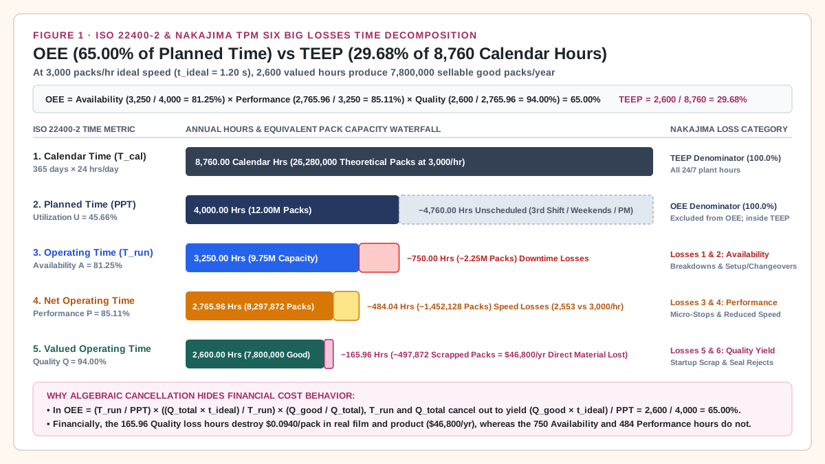
Takeaway: The overall equipment effectiveness formula reduces to Valued Operating Time / Planned Production Time, but you must keep Availability, Performance, and Quality separate because only Quality losses destroy $0.0940/pack in physical packaging material and product.
Why vendor OEE calculators overstate savings: the GAAP overhead absorption fallacy
Most commercial OEE ROI calculators ask for three inputs—planned hours, hourly machine burden rate, and target OEE gain—and multiply the freed hours (or theoretical extra packs) by the full hourly rate. In managerial accounting, that calculation violates the differential cash flow principle established in OpenStax Principles of Managerial Accounting, Section 10.1 (Identify Relevant Information for Decision-Making) and Section 6.5 (Compare and Contrast Variable and Absorption Costing): sunk equipment depreciation, facility leases, and unchanged straight-time shift payroll do not leave the income statement when a machine finishes its schedule early.
To trace every dollar across the income statement and cash flow statement, establish this baseline packaging line profile.
Worked example. Replace each input with a quote or a measured figure from the plant before using the result.
- Schedule & Nameplate Speed:
PPT_0 = 4,000.00planned production hours/year (45.6621%of8,760calendar hours). Nameplate ideal rate isR_ideal = 50 packs/minute = 3,000 packs/hour(t_ideal = 1.20 seconds/pack), giving a theoretical maximum capacity in planned time ofQ_max = 12,000,000 packs/year. - Baseline OEE (
65.00%):Availability (A_0) = 81.25%(3,250.00actual operating hours;750.00hours lost to breakdowns and changeovers).Performance (P_0) = 85.1064%(2,553.1915attempted packs per operating hour vs3,000ideal, producingQ_total_0 = 8,297,872attempted packs/year, or2,765.96net speed hours).Quality (Q_0) = 94.00%(6.00%scrap rate, rejecting497,872packs/year and deliveringQ_good_0 = 7,800,000sellable good packs/year across2,600.00valued operating hours, orR_eff_0 = 1,950.00good packs/planned hour).
- Unit Price & True Variable Costs (classified per OpenStax Principles of Managerial Accounting, Section 2.2 (Cost Behavior Patterns)):
- Selling / Transfer Price (
P):$0.3000 / good pack($300.00 per 1,000 good packs). - Direct Material & Scrap Disposal (
c_mat):$0.0940 / attempted pack($0.0880pouch film, fitment, product fill, and corrugated case +$0.0060net scrap handling/disposal). At94.00%first-pass yield, effective material cost per good pack isAVC_mat_0 = $0.0940 / 0.9400 = $0.100000 / good pack($780,000.00/yearfor7,800,000good packs, comprising$733,200.00in shipped product and$46,800.00/yeardestroyed in the497,872scrapped packs). See Cost per Good Pack for why scrap belongs inside effective material cost. - Variable Machine Energy (
c_run):$12.00 / operating hourfor servo drives, thermal sealers, and compressed air while running ($39,000.00/yearacross3,250operating hours, or$0.005000 / good pack). - Total Baseline Unit Variable Cost (
AVC_0):$0.105000 / good pack($0.1000material +$0.0050variable energy), giving a bottleneck Unit Contribution Margin (CM_0) of$0.195000 / good pack($0.3000 - $0.1050).
- Selling / Transfer Price (
- Fixed & Straight-Time Conversion Pool (
$789,000.00/year):- Straight-Time Shift Crew (
L_fixed):3full-time operators ×$30.00/hourfully loaded straight-time wage =$90.00 / planned hour=$360,000.00/year($0.046154 / good packat7.8Mpacks). Under union or standard full-time employment policies, operators remain on regular40-hourweekly pay unless a whole shift is eliminated; see Labor Savings vs. Redeployment. When Saturday overtime is required, the statutory1.5×rate under 29 CFR § 778.107 (Fair Labor Standards Act Overtime Pay) increases crew cost to$135.00 / overtime hour(3 × $45.00/hr). - Committed Fixed Overhead (
TFC):$429,000.00/year($240,000/yearstraight-line equipment depreciation +$189,000/yearallocated floor space, property insurance, and fixed preventive maintenance contracts), equal to$107.25 / planned houror$0.055000 / good packat7.8Mnormal capacity. - Combined Fixed Conversion Rate:
$360,000 + $429,000 = $789,000.00/year, which equals$197.25 / planned houror$0.101154 / good packat7,800,000good packs/year.
- Straight-Time Shift Crew (
Anatomy of the $60,692 phantom absorption savings
Now raise line OEE by +5.00 percentage points from 65.00% to 70.00% (R_eff_1 = 3,000 × 0.70 = 2,100.00 good packs/planned hour, a +7.6923% relative throughput increase). As shown in Average Fixed Cost Formula, Cost Per Unit Calculator, and Operating Leverage and mandated by IFRS IAS 2 Inventories, Paragraph 13 (along with US GAAP ASC 330-10-30), fixed production overhead is allocated to units based on normal capacity.
If a vendor calculator assumes the line runs all 4,000 hours at 70.00% OEE (8,400,000 good packs/year), average fixed conversion cost per pack (AFC_conv = $789,000 / Q) drops from $0.101154/pack to $0.093929/pack (-$0.007225/pack):
Phantom_Unit_Savings   = ($789,000 / 7,800,000) - ($789,000 / 8,400,000)
                       = $0.10115385 - $0.09392857 = $0.00722527 / pack
Claimed_Annual_Savings = 8,400,000 × $0.00722527 = $60,692.31 / year
  (Equivalently: 600,000 extra packs × $0.10115385 baseline AFC = $60,692.31 / year)
Or, if the vendor calculator holds output fixed at 7,800,000 packs and prices the 285.71 freed planned hours (4,000.00 - 3,714.29) at the full hourly conversion burden ($197.25/hour), it claims:
Claimed_Hourly_Savings = 285.7143 freed hours × $197.25/hour = $56,357.14 / year
Both figures are accounting illusions whenever customer demand is capped at 7,800,000 packs and the 3 operators stay on straight-time payroll. Total fixed conversion cash paid out by treasury remains exactly $789,000.00/year before and after the OEE project. To keep period totals and per-unit averages from colliding, compare this with Fixed, Variable and Total Cost Formulas and Cost of Goods Manufactured Formula: A Packaging WIP Reconciliation.
Takeaway: Dividing unchanged fixed overhead ($789,000/yr) by more theoretical packs creates $60,692/year in paper absorption variance while saving $0.00 in actual fixed cash outlay.
The 3 financial regimes of a +5% OEE gain (65% to 70%)
To translate an OEE percentage increase (OEE_0 = 65.00% to OEE_1 = 70.00%, achieved here by improving Availability or Performance while holding Quality at 94.00%) into verified cash flow, classify the packaging line into one of three operating regimes before running the numbers.
Regime 1: Demand-constrained / excess capacity (Q_bar = 7,800,000 packs/year)
When annual customer orders are fixed at Q_bar = 7,800,000 good packs and the line already meets that volume inside its regular 4,000-hour two-shift schedule, raising OEE from 65.00% (1,950 good packs/planned hour) to 70.00% (2,100 good packs/planned hour) reduces required planned production hours by 7.1429%:
PPT_req(70% OEE) = 7,800,000 / 2,100 = 3,714.2857 planned hours/year
ΔPPT_saved       = 4,000.00 - 3,714.2857 = 285.7143 freed planned hours/year
                   = 4,000 × (1 - 0.65 / 0.70) = 4,000 × (1 / 14) = 285.7143 hours
- Fixed Overhead & Straight-Time Payroll Saved:
$0.00/year. The285.71freed hours become unscheduled idle time unless management lays off operators or consolidates shifts; see Allocate Manufacturing Overhead After Automation. - Raw Material & Scrap Cash Saved (under Uptime/Speed lever at
94%Quality):$0.00/year. Producing7,800,000good packs at94.00%yield still requires7,800,000 / 0.94 = 8,297,872attempted packs and still scraps497,872packs ($46,800/year). - Variable Machine Energy Saved: Powered operating hours drop by up to
250.00hours (from3,250to3,000operating hours when operators power down drives after finishing the schedule early), saving250 × $12.00/hr=$3,000.00/year($2,785.71/yearif achieved purely via faster cycle speed across3,017.86operating hours).
Regime 2: Shift / labor-constrained overtime elimination (Q_bar = 8,400,000 packs/year)
Suppose customer demand is fixed at Q_bar = 8,400,000 good packs/year. At 65.00% baseline OEE (1,950 good packs/planned hour), the 4,000 regular two-shift hours produce only 7,800,000 good packs. To cover the 600,000-pack deficit without missing shipments, the plant runs Saturday overtime shifts:
OT_Hours_Baseline = (8,400,000 - 7,800,000) / 1,950 = 600,000 / 1,950 = 307.6923 overtime hours/year
Under 29 CFR § 778.107, those 307.6923 overtime planned hours require 1.5× straight-time wages (3 operators × $45.00/hr = $135.00/overtime hour). Raising OEE to 70.00% (2,100 good packs/planned hour) enables the crew to produce all 8,400,000 good packs inside the 4,000 regular straight-time hours (4,000 × 2,100 = 8,400,000), eliminating Saturday overtime completely:
ΔCash_Overtime_Payroll = 307.6923 OT hours × $135.00/hr = $41,538.46 / year
ΔCash_Variable_Energy  = 250.00 fewer operating hours × $12.00/hr = $3,000.00 / year
Total_Regime_2_Cash    = $41,538.46 + $3,000.00 = $44,538.46 / year
For multi-step overtime and shift boundary modeling, pair this calculation with Variable Cost Formula: Packaging Line Examples Across Shift Limits.
Regime 3: Capacity-constrained TOC bottleneck and CapEx deferral
When the packaging line is the primary factory bottleneck and customer demand absorbs every additional unit at P = $0.3000/pack, running all 4,000 planned hours at 70.00% OEE increases annual shipped output by ΔQ_good = +600,000 good packs/year (from 7,800,000 to 8,400,000).
-
Incremental Annual Operating Cash Flow (
ΔEBITDA): Following OpenStax Principles of Managerial Accounting, Section 3.2 (Break-Even Point and Contribution Margin), fixed costs ($789,000/yr) are already covered by baseline volume, so every incremental good pack generatesP - AVC_0in operating income. When the+5.00%OEE gain comes from Availability (Arising from81.25%to87.50%, adding250operating hours inside the4,000planned hours):ΔRevenue = +600,000 good packs × $0.3000/pack = +$180,000.00 / year ΔMaterial_Cost = +600,000 good packs × ($0.0940/0.94)= -$60,000.00 / year (638,298 attempts) ΔVariable_Energy = +250.00 operating hrs × $12.00/hr = -$3,000.00 / year ΔEBITDA_Regime_3 = +600,000 × $0.1950/pack = +$117,000.00 / year(If the
+5.00%OEE gain comes from Performance speed inside the existing3,250operating hours, variable running hours do not increase, liftingΔEBITDAto+$120,000.00/year.) -
Present Value of Deferred Capital Expenditure (
ΔNPV_CapEx): Suppose order volume is growing by300,000good packs/year (3.85%of baseline) and management was scheduled to spendCapEx = $1,500,000today on a parallel packaging line to avoid turning away orders. Unlocking+600,000good packs/year of bottleneck capacity on the existing line delays that$1,500,000capital outlay byn = 2.0years. Using the discounted cash flow formula in OpenStax Principles of Managerial Accounting, Section 11.4 (Use Discounted Cash Flow Models to Make Capital Investment Decisions) at a corporate cost of capital ofWACC = 10.00%:ΔNPV_CapEx = CapEx × [ 1 - (1 + WACC)^(-n) ] = $1,500,000 × [ 1 - (1.10)^(-2) ] = $1,500,000 × (1 - 0.82644628) = +$260,330.58 in present-value capital savingsIf the
+5.00%OEE gain defers the$1.5Mline byn = 3.0years,ΔNPV_CapExrises to+$373,027.80. Compare this capital-avoidance mechanism with How Equipment Utilization Changes Automation Payback.
Three-regime P&L and cash reconciliation table
Worked example. Replace each input with a quote or a measured figure from the plant before using the result.
Scroll horizontally to see all columns.
| Financial & Operational Line Item | Baseline (65.00% OEE at 7.8M) |
Vendor Calculator Fallacy (70% OEE) |
Regime 1: Excess Capacity (70% OEE, 7.8M Cap) |
Regime 2: Overtime Cut (65% → 70% at 8.4M Cap) |
Regime 3: Bottleneck (70% OEE, 8.4M Sold) |
|---|---|---|---|---|---|
1. Annual Sold Good Packs (Q_good) |
7,800,000 |
8,400,000 (assumed) |
7,800,000 |
8,400,000 |
8,400,000 (+600,000) |
2. Regular Straight-Time Hours (PPT) |
4,000.00 hrs |
4,000.00 hrs |
3,714.29 hrs (285.71 idle) |
4,000.00 hrs (was 4,000) |
4,000.00 hrs |
3. Saturday Overtime Hours (1.5×) |
0.00 hrs |
0.00 hrs |
0.00 hrs |
0.00 hrs (was 307.69 hrs) |
0.00 hrs |
4. Annual Revenue (P = $0.3000/pack) |
$2,340,000.00 |
N/A (cost-only) | $2,340,000.00 |
$2,520,000.00 (unchanged) |
$2,520,000.00 (+$180,000) |
5. Direct Material & Scrap (94% Yield) |
$780,000.00 |
$780,000.00 |
$780,000.00 ($0 saved) |
$840,000.00 ($0 saved) |
$840,000.00 (+$60,000 cost) |
6. Variable Machine Energy ($12/op-hr) |
$39,000.00 |
$39,000.00 |
$36,000.00 ($3,000 saved) |
$39,000.00 ($3,000 saved) |
$42,000.00 (+$3,000 via A) |
7. Straight-Time Crew Payroll ($360k) |
$360,000.00 |
Claims -$25,714 |
$360,000.00 ($0 saved) |
$360,000.00 ($0 change) |
$360,000.00 ($0 change) |
8. Overtime Crew Payroll ($135/OT-hr) |
$0.00 |
$0.00 |
$0.00 |
$0.00 ($41,538.46 saved) |
$0.00 |
9. Committed Fixed Overhead (TFC) |
$429,000.00 |
Claims -$34,978 |
$429,000.00 ($0 saved) |
$429,000.00 ($0 change) |
$429,000.00 ($0 change) |
| 10. Verified Annual Operating Cash Gain | Baseline | $60,692 (Phantom) |
+$3,000.00 / yr |
+$44,538.46 / yr |
+$117,000.00 / yr (+$120k via P) |
11. CapEx Deferral Present Value (ΔNPV) |
$0.00 |
$0.00 |
$0.00 |
$0.00 |
+$260,330.58 (2-yr delay) |
| 12. Total Year-1 Verified Economic Value | Baseline | Fails Audit | +$3,000.00 |
+$44,538.46 |
+$377,330.58 (EBITDA + ΔNPV) |
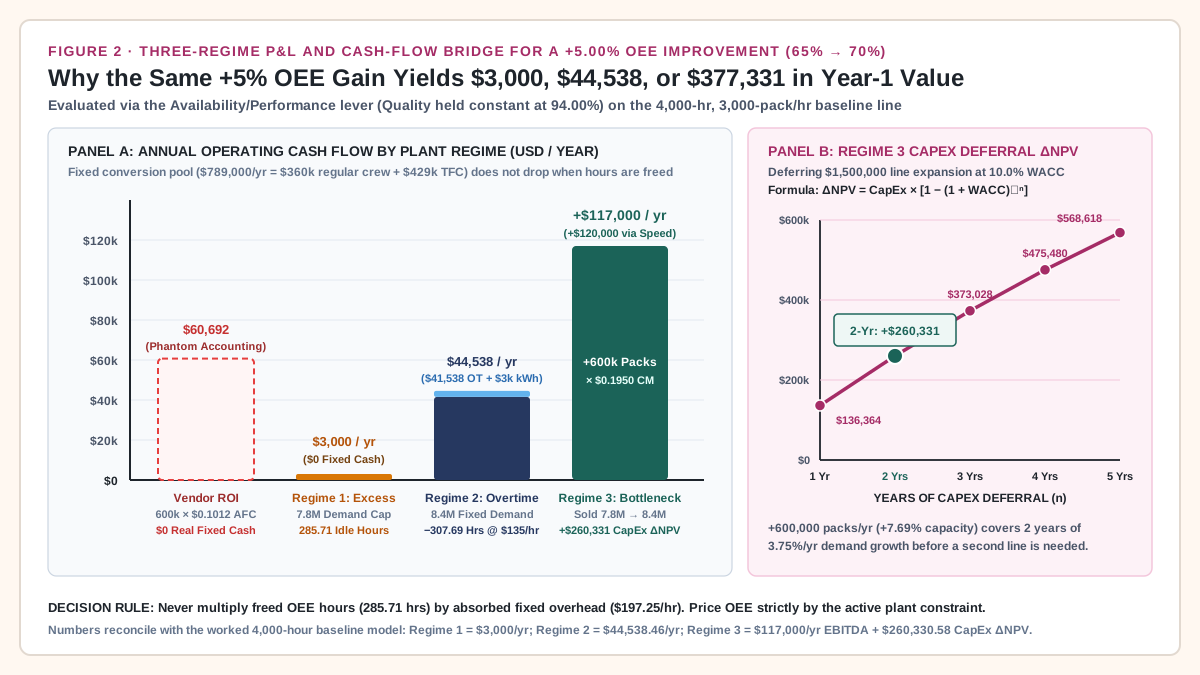
Takeaway: A +5.00% OEE improvement via uptime or speed generates $3,000/year in an excess-capacity plant, $44,538/year when it eliminates Saturday overtime, and +$117,000/year in EBITDA plus +$260,331 in deferred CapEx NPV on a true market-unconstrained bottleneck.
Component-specific financial impact: ΔAvailability vs ΔPerformance vs ΔQuality
Treating a +5.00% OEE gain from faster cycle speed (Performance) as financially identical to a +5.00% OEE gain from lower scrap (Quality) misallocates engineering capital in non-bottleneck plants. Even when customer orders are strictly capped at Q_bar = 7,800,000 good packs/year (Regime 1), improving the Quality factor saves hard cash on every single cycle by reducing total attempted packs (Q_total = Q_bar / Q).
Exact derivation of Quality yield cash savings (94.00% to 99.00%)
Suppose an engineering project installs closed-loop checkweigher feedback and servo-controlled heat-seal jaws, raising first-pass Quality (Q) from 94.00% (6.00% reject rate) to 99.00% (1.00% reject rate) while a minor speed/uptime tune brings compound OEE from 65.00% to 70.00% (0.8125 × 0.8703 × 0.9900 = 70.00%).
At fixed customer demand of Q_bar = 7,800,000 sellable good packs/year:
- At
94.00%Baseline Quality (Q_0 = 0.94):Q_total_0 = 7,800,000 / 0.94 = 8,297,872.34 attempted packs/year Q_scrap_0 = 8,297,872.34 - 7,800,000 = 497,872.34 rejected packs/year Material_Bill_0 = 8,297,872.34 × $0.0940 = $780,000.00 / year ($0.100000 / good pack) - At
99.00%Improved Quality (Q_1 = 0.99):Q_total_1 = 7,800,000 / 0.99 = 7,878,787.88 attempted packs/year Q_scrap_1 = 7,878,787.88 - 7,800,000 = 78,787.88 rejected packs/year Material_Bill_1 = 7,878,787.88 × $0.0940 = $740,606.06 / year ($0.094949 / good pack) - Net Annual Scrap & Energy Cash Saved at
7,800,000Good Packs:ΔScrap_Units_Eliminated = 497,872.34 - 78,787.88 = 419,084.46 fewer scrapped packs/year (-84.17%) ΔMaterial_Cash_Saved = 7,800,000 × $0.0940 × ( (1 / 0.94) - (1 / 0.99) ) = $780,000.00 - $740,606.06 = $39,393.94 / year ΔEnergy_Cash_Saved = (3,250.00 - 3,081.65 op hrs) × $12.00/hr = $2,020.20 / year Total_Regime_1_Quality = $39,393.94 + $2,020.20 = $41,414.14 / year
At 8,400,000 good packs/year (Regimes 2 and 3), raising Quality from 94.00% (8,936,170 attempts; 536,170 rejects) to 99.00% (8,484,848 attempts; 84,848 rejects) eliminates 451,322 scrapped packs/year, adding $42,424.24/year in direct material savings on top of the overtime payroll or bottleneck contribution margin gains! Compare how unplanned stops and changeover scrap behave in Measuring the Cost of Unplanned Production Downtime and Small Batches and Frequent Changeovers.
3x3 OEE lever vs plant regime cash matrix
Worked example. Replace each input with a quote or a measured figure from the plant before using the result.
Scroll horizontally to see all columns.
OEE Improvement Lever (65.00% → 70.00% Total OEE) |
Physical Change on the Line | Regime 1: Excess Capacity (7.8M Demand Cap) |
Regime 2: Overtime Elimination (8.4M Demand Cap) |
Regime 3: TOC Bottleneck (7.8M → 8.4M Sold) |
|---|---|---|---|---|
1. ΔAvailability Lever (A: 81.25% → 87.50%, P = 85.11%, Q = 94.00%) |
Cuts unplanned downtime & changeover stops; operating hours stay at 3,250 inside 3,714.29 planned hrs (Regime 1) or rise to 3,500 hrs in 4,000 PPT (Regimes 2 & 3). |
$0 – $3,000 / yr ($0 material, $0 fixed labor, $0–$3k standby power during 285.71 idle hrs) |
$41,538.46 / yr (307.69 OT hrs × $135/hr saved; operating hrs stay at 3,500, so $0 kWh delta) |
+$117,000.00 / yr EBITDA (+$180k rev -$60k mat -$3k extra kWh) + $260,330.58 CapEx ΔNPV |
2. ΔPerformance Lever (A = 81.25%, P: 85.11% → 91.65%, Q = 94.00%) |
Eliminates micro-stops & derating; lifts cycle rate from 2,553 to 2,750 attempts/op-hr (3,017.86 op hrs for 7.8M; 3,250 op hrs for 8.4M). |
$2,785.71 / yr ($0 material, $0 fixed labor, 232.14 fewer operating hrs × $12/hr kWh) |
$44,538.46 / yr ($41,538.46 OT payroll + 250.00 fewer OT operating hrs × $12/hr = $3,000 kWh) |
+$120,000.00 / yr EBITDA (+$180k rev -$60k mat, $0 extra kWh in 3,250 op hrs) + $260,330.58 CapEx ΔNPV |
3. ΔQuality Lever (Q: 94.00% → 99.00% + minor P/A to hit 70.00% OEE) |
Cuts reject rate from 6.00% to 1.00%, eliminating 419,084 scrapped packs at 7.8M (451,322 at 8.4M) and lowering AVC_mat from $0.1000 to $0.0949/pack. |
$41,414.14 / yr ($39,393.94 direct film/product scrap saved + $2,020.20 kWh saved) |
$86,962.70 / yr ($41,538.46 OT payroll + $3,000.00 kWh + $42,424.24 scrap saved at 8.4M) |
+$159,424.24 / yr EBITDA (+$117,000 CM + $42,424.24 scrap saved at 8.4M) + $260,330.58 CapEx ΔNPV |
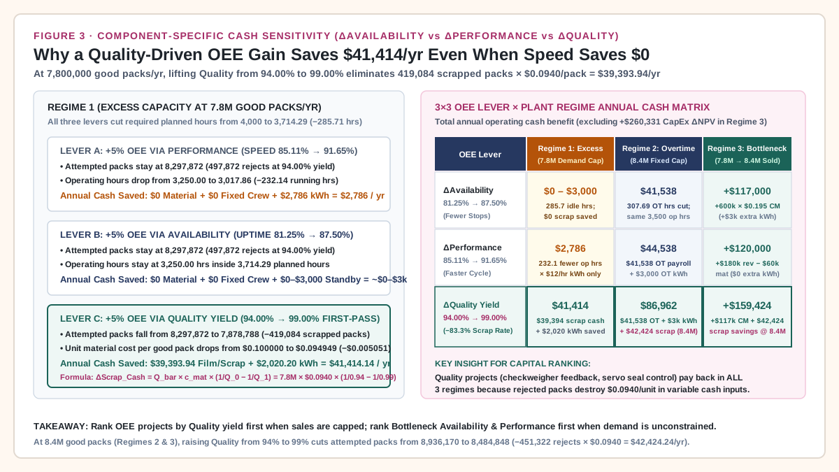
Takeaway: On any demand-constrained or non-bottleneck machine (Regime 1), target Quality yield (94% → 99%) first to capture $39,394/year in hard material savings; reserve Availability and Performance capital for lines running paid overtime (Regime 2) or limiting sold plant throughput (Regime 3).
Overall equipment effectiveness calculator and financial bridge in Excel
Build this 23-row overall equipment effectiveness calculator in Excel or Google Sheets (Cells B2:D24) to compute Availability, Performance, Quality, OEE, TEEP, freed planned hours, phantom vendor absorption claims, and verified cash flows across all three financial regimes. Keep raw numbers unformatted in inputs (Rows 2–17); Rows 18–24 reconcile every formula automatically. Pair this sheet with the Equipment ROI Spreadsheet when calculating multi-year Internal Rate of Return (IRR) and payback periods.
Worked example. Replace each input with a quote or a measured figure from the plant before using the result.
Scroll horizontally to see all columns.
| Row | Calculator Metric / Parameter | Col B: Baseline (65% OEE) Input or Formula |
Col C: Target (70% via Speed/Uptime) |
Col D: Target (70% via 99% Quality) |
|---|---|---|---|---|
| 2 | Calendar hours per year T_cal (hrs/yr) |
8760 |
8760 |
8760 |
| 3 | Planned production time PPT (hrs/yr) |
4000 |
4000 |
4000 |
| 4 | Actual operating time T_run (hrs/yr) |
3250 |
3500 |
3311.36 |
| 5 | Ideal cycle time t_ideal (seconds/pack) |
1.20 |
1.20 |
1.20 |
| 6 | Ideal nameplate rate R_ideal (packs/hr) |
=3600/B5 (3,000) |
=3600/C5 (3,000) |
=3600/D5 (3,000) |
| 7 | Total attempted units Q_total (packs/yr in 4,000 hrs) |
8297872.34 |
8936170.21 |
8484848.48 |
| 8 | Good sellable units Q_good (packs/yr in 4,000 hrs) |
7800000 |
8400000 |
8400000 |
| 9 | Availability (A = T_run / PPT) |
=B4/B3 (81.25%) |
=C4/C3 (87.50%) |
=D4/D3 (82.78%) |
| 10 | Performance (P = (Q_total × t_ideal) / (T_run × 3600)) |
=(B7*B5)/(B4*3600) (85.11%) |
=(C7*C5)/(C4*3600) (85.11%) |
=(D7*D5)/(D4*3600) (85.41%) |
| 11 | Quality (Q = Q_good / Q_total) |
=B8/B7 (94.00%) |
=C8/C7 (94.00%) |
=D8/D7 (99.00%) |
| 12 | Multiplicative OEE (A × P × Q) |
=B9*B10*B11 (65.00%) |
=C9*C10*C11 (70.00%) |
=D9*D10*D11 (70.00%) |
| 13 | Direct Ratio OEE Check ((Q_good × t_ideal) / (PPT × 3600)) |
=(B8*B5)/(B3*3600) (65.00%) |
=(C8*C5)/(C3*3600) (70.00%) |
=(D8*D5)/(D3*3600) (70.00%) |
| 14 | Calendar TEEP ((PPT / T_cal) × OEE) |
=(B3/B2)*B12 (29.68%) |
=(C3/C2)*C12 (31.96%) |
=(D3/D2)*D12 (31.96%) |
| 15 | Effective good rate R_eff (good packs / planned hr) |
=B6*B12 (1,950.00) |
=C6*C12 (2,100.00) |
=D6*D12 (2,100.00) |
| 16 | Unit inputs: Price P / Attempt Mat c_mat / Energy c_run |
0.3000 / 0.0940 / 12.00 |
0.3000 / 0.0940 / 12.00 |
0.3000 / 0.0940 / 12.00 |
| 17 | Fixed pool ($789,000) / OT Crew ($135/hr) / CapEx ($1.5M, 10%, 2 yr) |
789000 / 135 / 1500000 |
789000 / 135 / 1500000 |
789000 / 135 / 1500000 |
| 18 | Required PPT for 7.8M demand (= 7800000 / R_eff) |
=7800000/B15 (4,000.00 hrs) |
=7800000/C15 (3,714.29 hrs) |
=7800000/D15 (3,714.29 hrs) |
| 19 | Freed planned hours at 7.8M (= B18 - Col18) |
0.00 hrs |
=B18-C18 (285.71 hrs) |
=B18-D18 (285.71 hrs) |
| 20 | Vendor Phantom Absorption Claim (= (C8-B8)*(789000/B8)) |
$0.00 |
$60,692.31 / yr (Phantom) |
$60,692.31 / yr (Phantom) |
| 21 | Regime 1 Cash Saved (7.8M Cap: Scrap + Variable kWh) |
$0.00 |
$3,000.00 / yr ($0 fixed) |
$41,414.14 / yr ($39,394 scrap) |
| 22 | Regime 2 Cash Saved (8.4M Cap: 307.69 OT Hrs + kWh + Scrap) |
$0.00 |
$44,538.46 / yr ($41,538 OT) |
$86,962.70 / yr (+$42,424 scrap) |
| 23 | Regime 3 Bottleneck ΔEBITDA (+600k Sold Packs in 4,000 Hrs) |
$0.00 |
+$117,000.00 / yr (+$120k via P) |
+$159,424.24 / yr (CM + Scrap) |
| 24 | Regime 3 CapEx Deferral ΔNPV (= 1500000 * (1 - 1.10^-2)) |
$0.00 |
+$260,330.58 (2-yr delay) |
+$260,330.58 (2-yr delay) |
Verifying the spreadsheet formulas by hand
- Row 12 vs Row 13 Reconciliation: In Column B,
Availability × Performance × Quality = 0.8125 × 0.85106383 × 0.9400 = 0.6500(65.00%). Row 13 checks(7,800,000 × 1.20 seconds) / (4,000 hours × 3,600 seconds/hour) = 9,360,000 / 14,400,000 = 0.6500(65.00%). Any discrepancy between Row 12 and Row 13 flags an inconsistent cycle time (t_ideal) or unlogged rework count. - Row 21 (Regime 1 Cash Formula):
= 7800000 * 0.0940 * ((1 / B11) - (1 / D11)) + (B4 - (D4 * (7800000 / D8))) * 12.00 = $39,393.94 + $2,020.20 = $41,414.14 / year (in Column D) - Row 22 (Regime 2 Overtime Elimination Formula):
= ((8400000 - 7800000) / B15) * 135.00 + 3000.00 + 8400000 * 0.0940 * ((1 / B11) - (1 / D11))
= $41,538.46 + $3,000.00 + $42,424.24 = $86,962.70 / year (in Column D)
Takeaway: Always include both the Multiplicative OEE formula (Row 12) and the Direct Ratio OEE check (Row 13) in your spreadsheet, then link cash savings to the active regime row (Rows 21–24) instead of absorbed overhead (Row 20).
Common mistakes when translating OEE into financial ROI
Before presenting an OEE capital project to the plant controller or investment committee, audit the proposal against these five failure modes:
Scroll horizontally to see all columns.
| Failure Mode | Root Cause in Engineering Proposals | Financial or Operational Distortion | Controller & Engineering Prevention Rule |
|---|---|---|---|
| 1. Multiplying freed straight-time hours by full hourly burden | Pricing 285.71 freed planned hours at $197.25/hr ($90/hr regular crew + $107.25/hr fixed overhead). |
Invents $56,357–$60,692/yr in phantom savings when full-time operators and depreciation stay on the books. |
Credit labor cash savings only when verified overtime hours (1.5× FLSA rate), temporary agency contracts, or whole shifts are eliminated. |
2. Treating Speed (P) and Quality (Q) gains as equal in Regime 1 |
Using a single composite OEE percentage (65% → 70%) without specifying which of the three factors moved. |
Misses the $39,394/yr scrap cash difference between lifting Quality (94% → 99%) and lifting Performance speed ($0 material saved). |
Model ΔAvailability, ΔPerformance, and ΔQuality on separate lines so raw material and film scrap (c_mat / Q) is priced accurately. |
| 3. Averaging OEE across serial machines or upgrading a non-bottleneck | Spending capital to lift an upstream filler from 75% to 85% OEE when the downstream case packer limits the line at 65% OEE. |
Generates zero incremental shipped packs (ΔQ_good = 0) and zero overtime reduction on the line constraint; only increases accumulation jams. |
Measure and fund OEE improvements strictly at the primary Theory of Constraints (TOC) pacemaker station. |
4. Reclassifying changeover time out of PPT to inflate OEE |
Moving format changeovers and clean-in-place (CIP) stops from Availability losses into “unscheduled time” outside PPT. |
Artificially inflates reported OEE while actual Valued Operating Time (T_valued), TEEP, and good packs shipped fall. |
Lock PPT to total paid shift hours minus statutory breaks and track TEEP = T_valued / 8,760 alongside OEE on every monthly report. |
5. Approving parallel line CapEx at 65% OEE and 29.68% TEEP |
Ordering a $1,500,000 second packaging line when the existing machine runs two shifts with 750 downtime hours and 4,760 unscheduled calendar hours. |
Wastes $260,331–$373,028 in present-value capital cost (10% WACC) that a +5% bottleneck OEE fix or weekend crew shift would avoid. |
Require every capacity-expansion CapEx request to show baseline TEEP and prove why lifting bottleneck OEE by +5% cannot defer the purchase. |
Engineering rules of thumb for OEE capital allocation
- Rule of Thumb 1 (The Zero-Overtime Gate): If a packaging line logged fewer than
100overtime hours over the trailing12months and turns away zero customer orders (Regime 1), reject anyAvailabilityorPerformanceupgrade whose payback relies on labor or overhead absorption; approve onlyQualityyield upgrades whereQ_bar × c_mat × (1/Q_0 - 1/Q_1)pays back the investment in under24months. - Rule of Thumb 2 (The TEEP 35% CapEx Threshold): Never approve expansion CapEx for a parallel packaging machine when existing line
TEEPis below35.0%(3,066valued hours/year out of8,760) unless changeover frequency or customer delivery windows physically prevent adding shift hours or lifting bottleneckOEE. - Rule of Thumb 3 (Asymmetric Time vs Output Elasticity): Remember that a relative OEE increase from
OEE_0toOEE_1expands output at fixed hours by(OEE_1 / OEE_0) - 1(+7.6923%from65%to70%), but reduces required hours at fixed output by1 - (OEE_0 / OEE_1)(-7.1429%, or1/14). Never multiply baseline hours by+7.6923%when calculating freed shift time.
Return to the Production Economics reading guide to connect OEE financial bridges with unit cost curves, changeover batch sizing, and factory capacity utilization.
Takeaway: Audit every OEE proposal against the five failure modes above—separating phantom GAAP absorption from verified scrap reduction, overtime elimination, and bottleneck CapEx deferral before committing capital.
Frequently Asked Questions
What is the overall equipment effectiveness formula?
The overall equipment effectiveness formula is OEE = Availability × Performance × Quality, where Availability = Actual Operating Time / Planned Production Time (T_run / PPT), Performance = (Total Units Produced × Ideal Cycle Time) / Actual Operating Time ((Q_total × t_ideal) / T_run), and Quality = Good Units / Total Units Produced (Q_good / Q_total). Algebraically, T_run and Q_total cancel out to yield the direct ratio check OEE = (Q_good × t_ideal) / PPT = Valued Operating Time / Planned Production Time. On a packaging line with 4,000 planned hours and an ideal cycle time of 1.20 seconds/pack (3,000 packs/hour), 81.25% Availability × 85.11% Performance × 94.00% Quality equals 65.00% OEE (2,600 valued hours and 7,800,000 sellable good packs/year).
How do you calculate the financial impact of a 5% OEE improvement?
To calculate oee financial impact accurately, classify the line into one of three constraint regimes rather than multiplying freed hours by absorbed fixed overhead. In Regime 1 (Excess Capacity / Sales Capped at 7.8M packs), raising OEE from 65% to 70% frees 285.71 planned hours (4,000 × (1 - 0.65/0.70)), saving $0.00 in fixed depreciation or straight-time crew payroll and $0–$3,000/year in variable machine energy—unless the gain comes from lifting Quality (94% → 99%), which eliminates 419,084 scrapped packs and saves $39,393.94/year in raw material and film ($41,414.14/year with energy). In Regime 2 (Overtime Elimination at 8.4M packs), raising OEE from 65% (1,950 good packs/hr) to 70% (2,100 good packs/hr) fits all 8,400,000 packs inside 4,000 regular hours, eliminating 307.69 Saturday overtime hours at 1.5× FLSA wages ($135/hr) and saving $41,538.46/year in overtime payroll ($44,538.46/year with energy). In Regime 3 (TOC Bottleneck + CapEx Deferral), selling +600,000 incremental good packs at a unit contribution margin of $0.1950/pack ($0.3000 price minus $0.1050 variable cost) generates +$117,000/year in incremental EBITDA (+$159,424/year if achieved via 99% Quality), plus +$260,330.58 in present-value capital savings (ΔNPV = $1,500,000 × (1 - 1.10^-2)) by deferring a $1.5M parallel line expansion for 2 years at 10% WACC.
Why does a 5% OEE gain from Quality save more cash than a 5% gain from Performance speed on a non-bottleneck line?
When customer demand is capped (7,800,000 good packs/year in Regime 1) and full-time operators remain on straight-time payroll, running the machine faster (Performance) finishes the schedule 285.71 hours early but still requires 8,297,872 attempted cycles at 94.00% yield—destroying the exact same 497,872 rejected packs ($46,800/year in film and product) and saving only $2,785.71/year in drive electricity. By contrast, achieving the +5% OEE gain by raising Quality yield from 94.00% to 99.00% reduces total attempted cycles to 7,878,788 (78,788 rejects), eliminating 419,084 scrapped packs and saving $39,393.94/year in direct packaging material and disposal cash plus $2,020.20/year in variable energy ($41,414.14/year total).
What is the difference between the OEE formula and the TEEP formula?
Both formulas use Valued Operating Time (Q_good × t_ideal) in the numerator, but they divide by different time denominators. OEE divides by Planned Production Time (PPT)—the hours the plant scheduled the line to run (4,000 hours/year in a two-shift plant, giving 2,600 / 4,000 = 65.00% OEE). TEEP (Total Effective Equipment Performance) divides by All Calendar Time (8,760 hours/year = 365 days × 24 hours), multiplying Schedule Utilization (PPT / 8,760 = 45.66%) by OEE (65.00%) to yield 29.68% TEEP (2,600 / 8,760). OEE measures execution efficiency during scheduled shifts, whereas TEEP reveals how much untapped night and weekend schedule capacity remains before buying another machine.
Why do vendor OEE calculators overstate annual cost savings?
Vendor OEE calculators routinely divide fixed period conversion costs (such as $240,000 in equipment depreciation, $189,000 in facility lease and insurance overhead, and $360,000 in regular straight-time operator wages = $789,000/year or $197.25/planned hour) by baseline output (7,800,000 packs = $0.101154/pack) and treat any reduction in GAAP average fixed cost per unit (AFC = TFC / Q) as cash savings. Under US GAAP (ASC 330-10-30) and IFRS (IAS 2.13), lowering absorbed fixed overhead per pack by $0.007225/pack at 70% OEE ($60,692.31/year across 8.4M packs) is an inventory allocation adjustment, not a cash reduction; actual fixed cash outflow remains $789,000.00/year unless paid overtime hours or shift headcount are physically cut.