 WonksAnonymous
Build a Multi-Year Equipment Cash-Flow Model in Excel
A five-year Excel sheet for equipment cash that changes by year, with a negative overhaul year, cumulative recovery, and NPV.
An average annual return is the wrong summary when one year costs more than it saves. Put each year on its own row, then read cumulative cash, a five-year ROI, and NPV from those same rows.
The constant-benefit case, with one annual figure every year, is in Automation Payback, ROI and TCO. This sheet is the next step: savings ramp up, year 3 spends more than it saves, and a residual arrives at the end.
The amounts below are an original teaching example. They are a demonstration, not a supplier quote, a market price, a benchmark, or a customer result. No machine model is named.
Scroll horizontally to see all columns.
| Year | Date | Operating cash flow | Capital cash flow | Net cash flow | Cumulative net cash |
|---|---|---|---|---|---|
| 0 | 2026-01-01 | $0 | -$80,000 | -$80,000 | -$80,000 |
| 1 | 2027-01-01 | $8,000 | $0 | $8,000 | -$72,000 |
| 2 | 2028-01-01 | $22,000 | $0 | $22,000 | -$50,000 |
| 3 | 2029-01-01 | -$6,000 | $0 | -$6,000 | -$56,000 |
| 4 | 2030-01-01 | $24,000 | $0 | $24,000 | -$32,000 |
| 5 | 2031-01-01 | $24,000 | $10,000 | $34,000 | $2,000 |
Takeaway: One row per cash date keeps the ramp, the overhaul, and the residual in the same model.
Fill the rows from incremental cash, not from a machine brochure
Each operating amount is incremental to the status quo, the base case of keeping the current method. NIST’s investment guide defines the period cash flow in an NPV this way: net cash inflow during the period relative to the status quo, and that inflow can be negative. The opening $80,000 stands in for the whole installed outlay. What belongs in that total is listed in the true installed cost of packaging automation. This demonstration does not split the $80,000 into freight, installation, or training, because those splits need your quote.
Year 1 is a ramp: $8,000 of incremental operating cash. Years 2, 4, and 5 use $22,000 or $24,000. Year 3 is -$6,000 because, in this demonstration, the overhaul payment is larger than that year’s savings. The -$6,000 is a cash item in the operating column. It is a teaching input, not a maintenance quote. The $10,000 in year 5 is a demonstration assumption that the machine is sold for cash on 2031-01-01 and that the status quo frees no offsetting cash. If the current method also releases cash then, enter only the difference.
Cash that still leaves the business does not belong in these cells. Hours that move to other work stay in payroll, which labor savings versus redeployment separates from cash that stops. If productive hours change, rewrite the operating cells. How equipment utilization changes payback shows that hour test on a constant annual benefit. This sheet does not convert hours into dollars for you.
Takeaway: Every operating cell is incremental cash versus the current method, and the opening cell is the installed outlay.
Lay the sheet out so the date and the formula stay visible
Enter the inputs in columns C and D. Let formulas build net cash, the cumulative total, and the later ratios. The formulas use commas between arguments, the separator in Excel set to English (United States). Installations that use semicolons as the list separator need semicolons in these formulas. Keep currency symbols in the cell format, not in the number you type.
Scroll horizontally to see all columns.
| Cell | Label | Entry |
|---|---|---|
| B1 | Chosen annual discount rate | 0.08 |
| A4 | Year 0 | 0 |
| B4 | Date | 2026-01-01 |
| C4 | Operating cash flow | 0 |
| D4 | Capital cash flow | -80000 |
| E4 | Net cash flow | =C4+D4 |
| F4 | Cumulative net cash | =E4 |
| A5:A9 | Years 1 to 5 | 1 through 5 |
| B5:B9 | Dates | 2027-01-01 through 2031-01-01 |
| C5:C9 | Operating cash flow | 8000, 22000, -6000, 24000, 24000 |
| D5:D8 | Capital cash flow | 0 |
| D9 | Residual cash | 10000 |
| E5 | Net cash flow | =C5+D5 (copy through E9) |
| F5 | Cumulative net cash | =F4+E5 (copy through F9) |
| G5 | Period cash return | =E5/ABS($D$4) (copy through G9) |
Leave G4 blank. The opening outlay is the denominator of the later ratios, not a period return of its own. Copying =E4/ABS($D$4) into G4 prints -100%, which is the outlay divided by itself.
Two checks close the sheet. F9 equals =SUM(E4:E9), and both equal 2,000. G5 through G9 equal 10%, 27.5%, -7.5%, 30%, and 42.5%.
The 8% in B1 is the rate this demonstration discounts with. It is not a cost of capital, a hurdle rate, or a market return. Replace it with the rate your own decision uses, and say which rate that is.
Takeaway: Inputs sit in the operating and capital columns. Net cash, cumulative cash, and the ratios are formulas.
Read cumulative cash before you quote a payback
Cumulative net cash is the running sum of the net cash column, including the opening outlay. On this sheet it moves from -$80,000 to -$72,000, then to -$50,000. Year 3 takes it back to -$56,000. Year 4 leaves it at -$32,000. Only the year-5 net cash of $34,000, which includes the $10,000 residual, brings the running sum to $2,000.
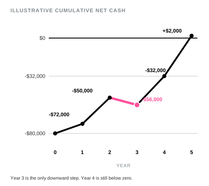
Dividing the opening outlay by the average later cash flow gives a different story. The five later net cash flows sum to $82,000, so the average is $16,400. Then $80,000 / $16,400 = 4.88 years. That division treats every year as if it paid $16,400. The cumulative column shows the year-3 reversal and shows that the project is still $32,000 unrecovered after four full years. The $10,000 residual is a lump on 2031-01-01, so this sheet does not split year 5 into a fractional payback month.
At a zero discount rate, NPV equals the sum of every net cash flow, including the opening outlay. Here that sum is $2,000, the same figure as F9. Use that equality as a check before you trust a discounted result.
Takeaway: Quote recovery from the cumulative column. An average-cash payback erases the year that steps backward.
Keep the period ratios separate from the five-year ROI
The five-year ROI uses the same ratio as the constant-benefit article: later net cash minus the opening outlay, divided by the opening outlay.
Five-year ROI = (SUM of net cash in years 1 to 5 - opening outlay) / opening outlay
             = (82,000 - 80,000) / 80,000
             = 2.5%
In the sheet that is =(SUM(E5:E9)+D4)/ABS(D4), because D4 is already stored as -80,000.
Scroll horizontally to see all columns.
| Result | Formula on this sheet | Value |
|---|---|---|
| Period cash returns | =E5/ABS($D$4) copied down |
10%, 27.5%, -7.5%, 30%, 42.5% |
| Average of those five ratios | =AVERAGE(E5:E9)/ABS($D$4) |
20.5% |
| Five-year ROI, residual included | =(SUM(E5:E9)+D4)/ABS(D4) |
2.5% |
| Five-year ROI, residual excluded | =(SUM(C5:C9)+D4)/ABS(D4) |
-10% |
| Price-path rate from $80,000 to $162,000 | =(162000/80000)^(1/5)-1 |
15.16% |
The 20.5% figure is the average later net cash divided by the opening outlay: $16,400 / $80,000. The 2.5% figure subtracts the opening outlay from the $82,000 sum before dividing. Drop the $10,000 residual and the operating cash sums to $72,000, so the five-year ROI is (72,000 - 80,000) / 80,000 = -10%. State whether the residual is inside the ROI.
The 15.16% figure is a compound annual growth rate on a made-up ending price. It takes $80,000 to $162,000, which is the opening outlay plus the $82,000 of later net cash, and asks what constant rate compounds across five years. Excel’s =RRI(5,80000,162000) answers that price-path question. The intermediate cash on this sheet is paid in or paid out on the dates above. Report the cumulative column, the 2.5% five-year ROI, and the NPV.
Takeaway: 20.5%, 2.5%, -10%, and 15.16% answer four different questions. Label the one you are reporting.
Add the opening outlay outside Excel’s NPV
Microsoft’s NPV function discounts a series of future payments and income. The values must be equally spaced and occur at the end of each period. The investment begins one period before the first value in the list. When the opening cash flow is paid at the start, add it to the NPV result. Leave it out of the values.
=D4+NPV(B1,E5:E9)
That expression is:
-80,000
+ 8,000 / 1.08
+ 22,000 / 1.08^2
+ (-6,000) / 1.08^3
+ 24,000 / 1.08^4
+ 34,000 / 1.08^5
= -17,713.59
The present value of the five later flows is $62,286.41. Subtracting the $80,000 outlay leaves -$17,713.59. At the 8% demonstration rate, NPV is negative even though the undiscounted running sum ends at +$2,000.
Putting the opening outlay inside NPV discounts it by one period and shifts every later flow out by one more period:
=NPV(B1,E4:E9)
= -80,000/1.08 + 8,000/1.08^2 + 22,000/1.08^3 + (-6,000)/1.08^4 + 24,000/1.08^5 + 34,000/1.08^6
= -16,401.47
Use the first formula when the machine is paid for on the start date.
NIST writes the same structure as Equation 4 in Appendix A of AMS 200-11: the discounted period cash flows, minus the initial investment cost. The guide’s own example uses a $200,000 outlay, later net cash flows of $22,000, $63,000, $45,000, $50,000, $56,000, and -$4,000, and a 4% discount rate. The present value of those later flows is $205,012.59, so NPV is $5,012.59. That published example is theirs. The five-year sheet on this page is a separate demonstration, and its NPV at 8% is negative.
IRR is the discount rate that sets this NPV to zero. NIST notes that the equation can return more than one rate when the algebra does so. These six cash flows change sign more than once. A scan of NPV from a -50% rate to a 75% rate crosses zero once, at about 0.68% (=IRR(E4:E9) on the six net-cash cells). Above that rate, NPV on this scan stays negative. Report NPV at the rate you chose, and treat a single IRR as the root you have checked.
Takeaway: =D4+NPV(B1,E5:E9) equals -$17,713.59 at 8%. The version that swallows the opening outlay equals -$16,401.47.
Use XNPV when a payment misses the period end
XNPV takes a discount rate, a series of cash flows, and the dates of those cash flows. The first value can be the opening cost, and a cost at the start is negative. Later amounts are discounted on a 365-day year. Every later date has to fall after the first date. For equally spaced period-end flows, Microsoft points you back to NPV.
=XNPV(B1,E4:E9,B4:B9)
On the annual dates in the table, that result is -$17,721.18. It differs from -$17,713.59 by $7.59 because 2028 is a leap year. The day counts from 2026-01-01 are 0, 365, 730, 1,096, 1,461, and 1,826. Equal-period NPV uses the exponents 1, 2, 3, 4, and 5. XNPV uses the day count divided by 365, so the last three flows sit slightly more than a whole number of years out.
Move only the -$6,000 overhaul from 2029-01-01 to 2028-07-01 and drop the empty 2029 date. The day count of 2028-07-01 is 912. XNPV on that dated series is -$17,909.56, about $188 further below the annual-date XNPV. NPV has no cell for 1 July. Use XNPV when the overhaul, the deposit, or the residual has a real date between period ends.
Takeaway: Annual dates make NPV and XNPV differ by $7.59 here. A 1 July overhaul belongs in XNPV, at -$17,909.56 on this demonstration.
Replace the demonstration with cash you can point to
Keep the row structure. Replace the amounts.
- Opening outlay: the installed total from the installed-cost list, not the machine price alone.
- Operating cash: payroll, overtime, or contract labor that actually stops, plus other cash that stops, minus new cash the machine adds. Labor savings versus redeployment is the test for the labor line.
- Hours: take them from your order book. When the hours change, change the operating cells. The utilization article linked above is the constant-benefit version of that test.
- Downtime: a downtime saving enters an operating cell only after you value it the way unplanned downtime cost does. Selling price is the wrong unit for an hour the line did not run.
- Rejects: fewer bad packs change cash once. Cost per good pack keeps that effect in the count of saleable output.
- Accounting totals: fixed, variable, and total cost reconciles operating costs for a period. A cost that continues under both the project and the status quo stays out of an incremental cell. Depreciation is an accounting allocation, not a row in this cash sheet, unless a tax payment changes the cash.
- Residual: cash you expect to receive, minus any residual the status quo would also release.
- After startup: replace the plan with measured cash. The 90-day post-installation review is built for that pass.
The Automation Investment guide collects the constant-benefit articles this sheet extends. The editorial policy states how this site treats worked examples.
Takeaway: The layout can stay. The dollars have to become your incremental cash, dated on the days the cash moves.
Frequently asked questions
How do I calculate ROI in Excel for multiple years when each year differs?
Sum the net cash flows after the opening outlay, subtract the opening outlay, and divide by the opening outlay. On this sheet that is =(SUM(E5:E9)+D4)/ABS(D4), which equals 2.5% with the residual included and -10% with the residual left out. Put the horizon next to the percentage.
Why does the average of the yearly ratios differ from the five-year ROI?
Each yearly ratio divides that year’s net cash by the opening outlay. Their average is 20.5%. The five-year ROI subtracts the opening outlay from the sum of the later cash flows before it divides, which produces 2.5% when the residual is included. Both figures are on the sheet. They are different results.
Where does the opening investment go in Excel’s NPV function?
Add the opening cash flow to the NPV result when it is paid at the start. The values inside NPV start with the first period-end flow. =D4+NPV(B1,E5:E9) equals -$17,713.59 at 8%. =NPV(B1,E4:E9) equals -$16,401.47 because it discounts the opening outlay.
When do I use XNPV instead of NPV?
Use XNPV when a cash flow has a date that is not the end of an equal period. On the annual dates here, XNPV is -$17,721.18. With the overhaul moved to 2028-07-01, XNPV is -$17,909.56. NPV still requires equal spacing and a period-end convention.
What do I do with a year whose net cash is negative?
Enter the negative amount in that year’s net cash cell. Cumulative cash steps backward by the same amount. In the demonstration, year 3 moves the running sum from -$50,000 to -$56,000, and the sum is still negative at the end of year 4.
Can I use CAGR for an equipment project?
CAGR, including Excel’s RRI, turns a starting value and an ending value into one annual rate. The 15.16% figure on this page is that rate from $80,000 to $162,000. The equipment results to report from this sheet are the cumulative cash, the five-year ROI, and NPV or XNPV on the dated flows.
Keep reading
- Automation Payback, ROI and TCO: payback, ROI, and TCO when the annual benefit is the same every year.
- The True Installed Cost of Packaging Automation: what to include before the opening cell is filled.
- How Equipment Utilization Changes Automation Payback: how fewer or more productive hours move a constant annual benefit.
Methods and sources
Updated October 11, 2026. WonksAnonymous Editors prepared this explanation with AI assistance. No independent audit of a factory’s books is claimed. Every dollar amount on the five-year sheet is an original illustrative calculation. The NIST example cited above is quoted from that guide and was recomputed from the net cash flows printed there: the present value of the later flows is $205,012.59 and the NPV is $5,012.59 at 4%.
Function behavior was checked against Microsoft’s documentation for NPV and XNPV: equal end-of-period spacing for NPV, the opening flow added outside NPV when it falls at the start, and a 365-day year for XNPV. The incremental-cash definition and Equation 4 are from NIST Advanced Manufacturing Series 200-11, Guide for Environmentally Sustainable Investment Analysis Based on ASTM E3200, Appendix A, PDF pages 25-26. This page states no machine model, speed, dimension, power rating, certification, or customer project.